The BetaML.Utils Module

Utils module

Provide shared utility functions and/or models for various machine learning algorithms.

For the complete list of functions provided see below. The main ones are:

Helper functions for logging

• Most BetaML functions accept a parameter verbosity (choose between NONE, LOW, STD, HIGH or FULL)
• Writing complex code and need to find where something is executed ? Use the macro @codelocation

Stochasticity management

• Utils provide [FIXEDSEED], [FIXEDRNG] and generate_parallel_rngs. All stochastic functions and models accept a rng parameter. See the "Getting started" section in the tutorial for details.

Data processing

• Various small and large utilities for helping processing the data, expecially before running a ML algorithm
• Includes getpermutations, OneHotEncoder, OrdinalEncoder, partition, Scaler, PCAEncoder, AutoEncoder, cross_validation.
• Auto-tuning of hyperparameters is implemented in the supported models by specifying autotune=true and optionally overriding the tunemethod parameters (e.g. for different hyperparameters ranges or different resources available for the tuning). Autotuning is then implemented in the (first) fit! call. Provided autotuning methods: SuccessiveHalvingSearch (default), GridSearch

Samplers

• Utilities to sample from data (e.g. for neural network training or for cross-validation)
• Include the "generic" type SamplerWithData, together with the sampler implementation KFold and the function batch

Transformers

• Funtions that "transform" a single input (that can be also a vector or a matrix)
• Includes varios NN "activation" functions (relu, celu, sigmoid, softmax, pool1d) and their derivatives (d[FunctionName]), but also gini, entropy, variance, BIC, AIC

Measures

• Several functions of a pair of parameters (often y and ŷ) to measure the goodness of ŷ, the distance between the two elements of the pair, ...
• Includes "classical" distance functions (l1_distance, l2_distance, l2squared_distance cosine_distance), "cost" functions for continuous variables (squared_cost, relative_mean_error) and comparision functions for multi-class variables (crossentropy, accuracy, ConfusionMatrix, silhouette)
• Distances can be used to compute a pairwise distance matrix using the function pairwise

mutable struct AutoE_hp <: BetaMLHyperParametersSet

Hyperparameters for the AutoEncoder transformer

Parameters

• encoded_size: The desired size of the encoded data, that is the number of dimensions in output or the size of the latent space. This is the number of neurons of the layer sitting between the econding and decoding layers. If the value is a float it is considered a percentual (to be rounded) of the dimensionality of the data [def: 0.33]

• layers_size: Inner layers dimension (i.e. number of neurons). If the value is a float it is considered a percentual (to be rounded) of the dimensionality of the data [def: nothing that applies a specific heuristic]. Consider that the underlying neural network is trying to predict multiple values at the same times. Normally this requires many more neurons than a scalar prediction. If e_layers or d_layers are specified, this parameter is ignored for the respective part.

• e_layers: The layers (vector of AbstractLayers) responsable of the encoding of the data [def: nothing, i.e. two dense layers with the inner one of layers_size]

• d_layers: The layers (vector of AbstractLayers) responsable of the decoding of the data [def: nothing, i.e. two dense layers with the inner one of layers_size]

• loss: Loss (cost) function [def: squared_cost] It must always assume y and ŷ as (n x d) matrices, eventually using dropdims inside.

• dloss: Derivative of the loss function [def: dsquared_cost if loss==squared_cost, nothing otherwise, i.e. use the derivative of the squared cost or autodiff]

• epochs: Number of epochs, i.e. passages trough the whole training sample [def: 200]

• batch_size: Size of each individual batch [def: 8]

• opt_alg: The optimisation algorithm to update the gradient at each batch [def: ADAM()]

• shuffle: Whether to randomly shuffle the data at each iteration (epoch) [def: true]

• tunemethod: The method - and its parameters - to employ for hyperparameters autotuning. See SuccessiveHalvingSearch for the default method. To implement automatic hyperparameter tuning during the (first) fit! call simply set autotune=true and eventually change the default tunemethod options (including the parameter ranges, the resources to employ and the loss function to adopt).

mutable struct AutoEncoder <: BetaMLUnsupervisedModel

Perform a (possibly-non linear) transformation ("encoding") of the data into a different space, e.g. for dimensionality reduction using neural network trained to replicate the input data.

A neural network is trained to first transform the data (ofter "compress") to a subspace (the output of an inner layer) and then retransform (subsequent layers) to the original data.

predict(mod::AutoEncoder,x) returns the encoded data, inverse_predict(mod::AutoEncoder,xtransformed) performs the decoding.

For the parameters see AutoE_hp and BML_options

Notes:

• AutoEncoder doesn't automatically scale the data. It is suggested to apply the Scaler model before running it.
• Missing data are not supported. Impute them first, see the Imputation module.
• Decoding layers can be optinally choosen (parameter d_layers) in order to suit the kind of data, e.g. a relu activation function for nonegative data

Example:

julia> using BetaML

julia> x = [0.12 0.31 0.29 3.21 0.21;
            0.22 0.61 0.58 6.43 0.42;
            0.51 1.47 1.46 16.12 0.99;
            0.35 0.93 0.91 10.04 0.71;
            0.44 1.21 1.18 13.54 0.85];

julia> m    = AutoEncoder(encoded_size=1,epochs=400)
A AutoEncoder BetaMLModel (unfitted)

julia> x_reduced = fit!(m,x)
***
*** Training  for 400 epochs with algorithm ADAM.
Training..       avg loss on epoch 1 (1):        60.27802763757111
Training..       avg loss on epoch 200 (200):    0.08970099870421573
Training..       avg loss on epoch 400 (400):    0.013138484118673664
Training of 400 epoch completed. Final epoch error: 0.013138484118673664.
5×1 Matrix{Float64}:
  -3.5483740608901186
  -6.90396890458868
 -17.06296512222304
 -10.688936344498398
 -14.35734756603212

julia> x̂ = inverse_predict(m,x_reduced)
5×5 Matrix{Float64}:
 0.0982406  0.110294  0.264047   3.35501  0.327228
 0.205628   0.470884  0.558655   6.51042  0.487416
 0.529785   1.56431   1.45762   16.067    0.971123
 0.3264     0.878264  0.893584  10.0709   0.667632
 0.443453   1.2731    1.2182    13.5218   0.842298

julia> info(m)["rme"]
0.020858783340281222

julia> hcat(x,x̂)
5×10 Matrix{Float64}:
 0.12  0.31  0.29   3.21  0.21  0.0982406  0.110294  0.264047   3.35501  0.327228
 0.22  0.61  0.58   6.43  0.42  0.205628   0.470884  0.558655   6.51042  0.487416
 0.51  1.47  1.46  16.12  0.99  0.529785   1.56431   1.45762   16.067    0.971123
 0.35  0.93  0.91  10.04  0.71  0.3264     0.878264  0.893584  10.0709   0.667632
 0.44  1.21  1.18  13.54  0.85  0.443453   1.2731    1.2182    13.5218   0.842298

mutable struct ConfusionMatrix <: BetaMLUnsupervisedModel

Compute a confusion matrix detailing the mismatch between observations and predictions of a categorical variable

For the parameters see ConfusionMatrix_hp and BML_options.

The "predicted" values are either the scores or the normalised scores (depending on the parameter normalise_scores [def: true]).

Notes:

• The Confusion matrix report can be printed (i.e. print(cm_model). If you plan to print the Confusion Matrix report, be sure that the type of the data in y and ŷ can be converted to String.

• Information in a structured way is available trought the info(cm) function that returns the following dictionary:

  • accuracy: Oveall accuracy rate
  • misclassification: Overall misclassification rate
  • actual_count: Array of counts per lebel in the actual data
  • predicted_count: Array of counts per label in the predicted data
  • scores: Matrix actual (rows) vs predicted (columns)
  • normalised_scores: Normalised scores
  • tp: True positive (by class)
  • tn: True negative (by class)
  • fp: False positive (by class)
  • fn: False negative (by class)
  • precision: True class i over predicted class i (by class)
  • recall: Predicted class i over true class i (by class)
  • specificity: Predicted not class i over true not class i (by class)
  • f1score: Harmonic mean of precision and recall
  • mean_precision: Mean by class, respectively unweighted and weighted by actual_count
  • mean_recall: Mean by class, respectively unweighted and weighted by actual_count
  • mean_specificity: Mean by class, respectively unweighted and weighted by actual_count
  • mean_f1score: Mean by class, respectively unweighted and weighted by actual_count
  • categories: The categories considered
  • fitted_records: Number of records considered
  • n_categories: Number of categories considered

Example:

The confusion matrix can also be plotted, e.g.:

julia> using Plots, BetaML

julia> y  = ["apple","mandarin","clementine","clementine","mandarin","apple","clementine","clementine","apple","mandarin","clementine"];

julia> ŷ  = ["apple","mandarin","clementine","mandarin","mandarin","apple","clementine","clementine",missing,"clementine","clementine"];

julia> cm = ConfusionMatrix(handle_missing="drop")
A ConfusionMatrix BetaMLModel (unfitted)

julia> normalised_scores = fit!(cm,y,ŷ)
3×3 Matrix{Float64}:
 1.0  0.0       0.0
 0.0  0.666667  0.333333
 0.0  0.2       0.8

julia> println(cm)
A ConfusionMatrix BetaMLModel (fitted)

-----------------------------------------------------------------

*** CONFUSION MATRIX ***

Scores actual (rows) vs predicted (columns):

4×4 Matrix{Any}:
 "Labels"       "apple"   "mandarin"   "clementine"
 "apple"       2         0            0
 "mandarin"    0         2            1
 "clementine"  0         1            4
Normalised scores actual (rows) vs predicted (columns):

4×4 Matrix{Any}:
 "Labels"       "apple"   "mandarin"   "clementine"
 "apple"       1.0       0.0          0.0
 "mandarin"    0.0       0.666667     0.333333
 "clementine"  0.0       0.2          0.8

 *** CONFUSION REPORT ***

- Accuracy:               0.8
- Misclassification rate: 0.19999999999999996
- Number of classes:      3

  N Class      precision   recall  specificity  f1score  actual_count  predicted_count
                             TPR       TNR                 support                  

  1 apple          1.000    1.000        1.000    1.000            2               2
  2 mandarin       0.667    0.667        0.857    0.667            3               3
  3 clementine     0.800    0.800        0.800    0.800            5               5

- Simple   avg.    0.822    0.822        0.886    0.822
- Weigthed avg.    0.800    0.800        0.857    0.800

-----------------------------------------------------------------
Output of `info(cm)`:
- mean_precision:       (0.8222222222222223, 0.8)
- fitted_records:       10
- specificity:  [1.0, 0.8571428571428571, 0.8]
- precision:    [1.0, 0.6666666666666666, 0.8]
- misclassification:    0.19999999999999996
- mean_recall:  (0.8222222222222223, 0.8)
- n_categories: 3
- normalised_scores:    [1.0 0.0 0.0; 0.0 0.6666666666666666 0.3333333333333333; 0.0 0.2 0.8]
- tn:   [8, 6, 4]
- mean_f1score: (0.8222222222222223, 0.8)
- actual_count: [2, 3, 5]
- accuracy:     0.8
- recall:       [1.0, 0.6666666666666666, 0.8]
- f1score:      [1.0, 0.6666666666666666, 0.8]
- mean_specificity:     (0.8857142857142858, 0.8571428571428571)
- predicted_count:      [2, 3, 5]
- scores:       [2 0 0; 0 2 1; 0 1 4]
- tp:   [2, 2, 4]
- fn:   [0, 1, 1]
- categories:   ["apple", "mandarin", "clementine"]
- fp:   [0, 1, 1]

julia> res = info(cm);

julia> heatmap(string.(res["categories"]),string.(res["categories"]),res["normalised_scores"],seriescolor=cgrad([:white,:blue]),xlabel="Predicted",ylabel="Actual", title="Confusion Matrix (normalised scores)")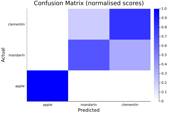

mutable struct ConfusionMatrix_hp <: BetaMLHyperParametersSet

Hyperparameters for ConfusionMatrix

Parameters:

• categories: The categories (aka "levels") to represent. [def: nothing, i.e. unique ground true values].

• handle_unknown: How to handle categories not seen in the ground true values or not present in the provided categories array? "error" (default) rises an error, "infrequent" adds a specific category for these values.

• handle_missing: How to handle missing values in either ground true or predicted values ? "error" [default] will rise an error, "drop" will drop the record

• other_categories_name: Which value to assign to the "other" category (i.e. categories not seen in the gound truth or not present in the provided categories array? [def: nothing, i.e. typemax(Int64) for integer vectors and "other" for other types]. This setting is active only if handle_unknown="infrequent" and in that case it MUST be specified if the vector to one-hot encode is neither integer or strings

• categories_names: A dictionary to map categories to some custom names. Useful for example if categories are integers, or you want to use shorter names [def: Dict(), i.e. not used]. This option isn't currently compatible with missing values or when some record has a value not in this provided dictionary.

• normalise_scores: Wether predict should return the normalised scores. Note that both unnormalised and normalised scores remain available using info. [def: true]

mutable struct GridSearch <: AutoTuneMethod

Simple grid method for hyper-parameters validation of supervised models.

All parameters are tested using cross-validation and then the "best" combination is used.

Notes:

• the default loss is suitable for 1-dimensional output supervised models

Parameters:

• loss::Function: Loss function to use. [def: l2loss_by_cv]. Any function that takes a model, data (a vector of arrays, even if we work only with X) and (using therng` keyword) a RNG and return a scalar loss.

• res_share::Float64: Share of the (data) resources to use for the autotuning [def: 0.1]. With res_share=1 all the dataset is used for autotuning, it can be very time consuming!

• hpranges::Dict{String, Any}: Dictionary of parameter names (String) and associated vector of values to test. Note that you can easily sample these values from a distribution with rand(distrobject,nvalues). The number of points you provide for a given parameter can be interpreted as proportional to the prior you have on the importance of that parameter for the algorithm quality.

• multithreads::Bool: Use multithreads in the search for the best hyperparameters [def: false]

KFold(nsplits=5,nrepeats=1,shuffle=true,rng=Random.GLOBAL_RNG)

Iterator for k-fold cross_validation strategy.

mutable struct MinMaxScaler <: BetaML.Utils.AbstractScaler

Scale the data to a given (def: unit) hypercube

Parameters:

• inputRange: The range of the input. [def: (minimum,maximum)]. Both ranges are functions of the data. You can consider other relative of absolute ranges using e.g. inputRange=(x->minimum(x)*0.8,x->100)

• outputRange: The range of the scaled output [def: (0,1)]

Example:

julia> using BetaML

julia> x       = [[4000,1000,2000,3000] ["a", "categorical", "variable", "not to scale"] [4,1,2,3] [0.4, 0.1, 0.2, 0.3]]
4×4 Matrix{Any}:
 4000  "a"             4  0.4
 1000  "categorical"   1  0.1
 2000  "variable"      2  0.2
 3000  "not to scale"  3  0.3

julia> mod     = Scaler(MinMaxScaler(outputRange=(0,10)), skip=[2])
A Scaler BetaMLModel (unfitted)

julia> xscaled = fit!(mod,x)
4×4 Matrix{Any}:
 10.0      "a"             10.0      10.0
  0.0      "categorical"    0.0       0.0
  3.33333  "variable"       3.33333   3.33333
  6.66667  "not to scale"   6.66667   6.66667

julia> xback   = inverse_predict(mod, xscaled)
4×4 Matrix{Any}:
 4000.0  "a"             4.0  0.4
 1000.0  "categorical"   1.0  0.1
 2000.0  "variable"      2.0  0.2
 3000.0  "not to scale"  3.0  0.3

mutable struct OneHotE_hp <: BetaMLHyperParametersSet

Hyperparameters for both OneHotEncoder and OrdinalEncoder

Parameters:

• categories: The categories to represent as columns. [def: nothing, i.e. unique training values or range for integers]. Do not include missing in this list.

• handle_unknown: How to handle categories not seen in training or not present in the provided categories array? "error" (default) rises an error, "missing" labels the whole output with missing values, "infrequent" adds a specific column for these categories in one-hot encoding or a single new category for ordinal one.

• other_categories_name: Which value during inverse transformation to assign to the "other" category (i.e. categories not seen on training or not present in the provided categories array? [def: nothing, i.e. typemax(Int64) for integer vectors and "other" for other types]. This setting is active only if handle_unknown="infrequent" and in that case it MUST be specified if the vector to one-hot encode is neither integer or strings

mutable struct OneHotEncoder <: BetaMLUnsupervisedModel

Encode a vector of categorical values as one-hot columns.

The algorithm distinguishes between missing values, for which it returns a one-hot encoded row of missing values, and other categories not in the provided list or not seen during training that are handled according to the handle_unknown parameter.

For the parameters see OneHotE_hp and BML_options. This model supports inverse_predict.

Example:

julia> using BetaML

julia> x       = ["a","d","e","c","d"];

julia> mod     = OneHotEncoder(handle_unknown="infrequent",other_categories_name="zz")
A OneHotEncoder BetaMLModel (unfitted)

julia> x_oh    = fit!(mod,x)  # last col is for the "infrequent" category
5×5 Matrix{Bool}:
 1  0  0  0  0
 0  1  0  0  0
 0  0  1  0  0
 0  0  0  1  0
 0  1  0  0  0

julia> x2      = ["a","b","c"];

julia> x2_oh   = predict(mod,x2)
3×5 Matrix{Bool}:
 1  0  0  0  0
 0  0  0  0  1
 0  0  0  1  0

julia> x2_back = inverse_predict(mod,x2_oh)
3-element Vector{String}:
 "a"
 "zz"
 "c"

mutable struct OrdinalEncoder <: BetaMLUnsupervisedModel

Encode a vector of categorical values as integers.

The algorithm distinguishes between missing values, for which it propagate the missing, and other categories not in the provided list or not seen during training that are handled according to the handle_unknown parameter.

For the parameters see OneHotE_hp and BML_options. This model supports inverse_predict.

Example:

julia> using BetaML

julia> x       = ["a","d","e","c","d"];

julia> mod     = OrdinalEncoder(handle_unknown="infrequent",other_categories_name="zz")
A OrdinalEncoder BetaMLModel (unfitted)

julia> x_int   = fit!(mod,x)
5-element Vector{Int64}:
 1
 2
 3
 4
 2

julia> x2      = ["a","b","c","g"];

julia> x2_int  = predict(mod,x2) # 5 is for the "infrequent" category
4-element Vector{Int64}:
 1
 5
 4
 5

julia> x2_back = inverse_predict(mod,x2_oh)
4-element Vector{String}:
 "a"
 "zz"
 "c"
 "zz"

mutable struct PCAE_hp <: BetaMLHyperParametersSet

Hyperparameters for the PCAEncoder transformer

Parameters

• encoded_size: The size, that is the number of dimensions, to maintain (with encoded_size <= size(X,2) ) [def: nothing, i.e. the number of output dimensions is determined from the parameter max_unexplained_var]

• max_unexplained_var: The maximum proportion of variance that we are willing to accept when reducing the number of dimensions in our data [def: 0.05]. It doesn't have any effect when the output number of dimensions is explicitly chosen with the parameter encoded_size

mutable struct PCAEncoder <: BetaMLUnsupervisedModel

Perform a Principal Component Analysis, a dimensionality reduction tecnique employing a linear trasformation of the original matrix by the eigenvectors of the covariance matrix.

PCAEncoder returns the matrix reprojected among the dimensions of maximum variance.

For the parameters see PCAE_hp and BML_options

Notes:

• PCAEncoder doesn't automatically scale the data. It is suggested to apply the Scaler model before running it.
• Missing data are not supported. Impute them first, see the Imputation module.
• If one doesn't know a priori the maximum unexplained variance that he is willling to accept, nor the wished number of dimensions, he can run the model with all the dimensions in output (i.e. with encoded_size=size(X,2)), analise the proportions of explained cumulative variance by dimensions in info(mod,""explained_var_by_dim"), choose the number of dimensions K according to his needs and finally pick from the reprojected matrix only the number of dimensions required, i.e. out.X[:,1:K].

Example:

julia> using BetaML

julia> xtrain        = [1 10 100; 1.1 15 120; 0.95 23 90; 0.99 17 120; 1.05 8 90; 1.1 12 95];

julia> mod           = PCAEncoder(max_unexplained_var=0.05)
A PCAEncoder BetaMLModel (unfitted)

julia> xtrain_reproj = fit!(mod,xtrain)
6×2 Matrix{Float64}:
 100.449    3.1783
 120.743    6.80764
  91.3551  16.8275
 120.878    8.80372
  90.3363   1.86179
  95.5965   5.51254

julia> info(mod)
Dict{String, Any} with 5 entries:
  "explained_var_by_dim" => [0.873992, 0.999989, 1.0]
  "fitted_records"       => 6
  "prop_explained_var"   => 0.999989
  "retained_dims"        => 2
  "xndims"               => 3

julia> xtest         = [2 20 200];

julia> xtest_reproj  = predict(mod,xtest)
1×2 Matrix{Float64}:
 200.898  6.3566

SamplerWithData{Tsampler}

Associate an instance of an AbstractDataSampler with the actual data to sample.

mutable struct Scaler <: BetaMLUnsupervisedModel

Scale the data according to the specific chosen method (def: StandardScaler)

For the parameters see Scaler_hp and BML_options

Examples:

• Standard scaler (default)...

julia> using BetaML, Statistics

julia> x         = [[4000,1000,2000,3000] [400,100,200,300] [4,1,2,3] [0.4, 0.1, 0.2, 0.3]]
4×4 Matrix{Float64}:
 4000.0  400.0  4.0  0.4
 1000.0  100.0  1.0  0.1
 2000.0  200.0  2.0  0.2
 3000.0  300.0  3.0  0.3

julia> mod       = Scaler() # equiv to `Scaler(StandardScaler(scale=true, center=true))`
A Scaler BetaMLModel (unfitted)

julia> xscaled   = fit!(mod,x)
4×4 Matrix{Float64}:
  1.34164    1.34164    1.34164    1.34164
 -1.34164   -1.34164   -1.34164   -1.34164
 -0.447214  -0.447214  -0.447214  -0.447214
  0.447214   0.447214   0.447214   0.447214

julia> col_means = mean(xscaled, dims=1)
1×4 Matrix{Float64}:
 0.0  0.0  0.0  5.55112e-17

julia> col_var   = var(xscaled, dims=1, corrected=false)
1×4 Matrix{Float64}:
 1.0  1.0  1.0  1.0

julia> xback     = inverse_predict(mod, xscaled)
4×4 Matrix{Float64}:
 4000.0  400.0  4.0  0.4
 1000.0  100.0  1.0  0.1
 2000.0  200.0  2.0  0.2
 3000.0  300.0  3.0  0.3

• Min-max scaler...

julia> using BetaML

julia> x       = [[4000,1000,2000,3000] ["a", "categorical", "variable", "not to scale"] [4,1,2,3] [0.4, 0.1, 0.2, 0.3]]
4×4 Matrix{Any}:
 4000  "a"             4  0.4
 1000  "categorical"   1  0.1
 2000  "variable"      2  0.2
 3000  "not to scale"  3  0.3

julia> mod     = Scaler(MinMaxScaler(outputRange=(0,10)),skip=[2])
A Scaler BetaMLModel (unfitted)

julia> xscaled = fit!(mod,x)
4×4 Matrix{Any}:
 10.0      "a"             10.0      10.0
  0.0      "categorical"    0.0       0.0
  3.33333  "variable"       3.33333   3.33333
  6.66667  "not to scale"   6.66667   6.66667

julia> xback   = inverse_predict(mod,xscaled)
4×4 Matrix{Any}:
 4000.0  "a"             4.0  0.4
 1000.0  "categorical"   1.0  0.1
 2000.0  "variable"      2.0  0.2
 3000.0  "not to scale"  3.0  0.3

mutable struct Scaler_hp <: BetaMLHyperParametersSet

Hyperparameters for the Scaler transformer

Parameters

• method: The specific scaler method to employ with its own parameters. See StandardScaler [def] or MinMaxScaler.

• skip: The positional ids of the columns to skip scaling (eg. categorical columns, dummies,...) [def: []]

mutable struct StandardScaler <: BetaML.Utils.AbstractScaler

Standardise the input to zero mean and unit standard deviation, aka "Z-score". Note that missing values are skipped.

Parameters:

• scale: Scale to unit variance [def: true]

• center: Center to zero mean [def: true]

Example:

julia> using BetaML, Statistics

julia> x         = [[4000,1000,2000,3000] [400,100,200,300] [4,1,2,3] [0.4, 0.1, 0.2, 0.3]]
4×4 Matrix{Float64}:
 4000.0  400.0  4.0  0.4
 1000.0  100.0  1.0  0.1
 2000.0  200.0  2.0  0.2
 3000.0  300.0  3.0  0.3

julia> mod       = Scaler() # equiv to `Scaler(StandardScaler(scale=true, center=true))`
A Scaler BetaMLModel (unfitted)

julia> xscaled   = fit!(mod,x)
4×4 Matrix{Float64}:
  1.34164    1.34164    1.34164    1.34164
 -1.34164   -1.34164   -1.34164   -1.34164
 -0.447214  -0.447214  -0.447214  -0.447214
  0.447214   0.447214   0.447214   0.447214

julia> col_means = mean(xscaled, dims=1)
1×4 Matrix{Float64}:
 0.0  0.0  0.0  5.55112e-17

julia> col_var   = var(xscaled, dims=1, corrected=false)
1×4 Matrix{Float64}:
 1.0  1.0  1.0  1.0

julia> xback     = inverse_predict(mod, xscaled)
4×4 Matrix{Float64}:
 4000.0  400.0  4.0  0.4
 1000.0  100.0  1.0  0.1
 2000.0  200.0  2.0  0.2
 3000.0  300.0  3.0  0.3

mutable struct SuccessiveHalvingSearch <: AutoTuneMethod

Hyper-parameters validation of supervised models that search the parameters space trouth successive halving

All parameters are tested on a small sub-sample, then the "best" combinations are kept for a second round that use more samples and so on untill only one hyperparameter combination is left.

Notes:

• the default loss is suitable for 1-dimensional output supervised models, and applies itself cross-validation. Any function that accepts a model, some data and return a scalar loss can be used
• the rate at which the potential candidate combinations of hyperparameters shrink is controlled by the number of data shares defined in res_shared (i.e. the epochs): more epochs are choosen, lower the "shrink" coefficient

Parameters:

• loss::Function: Loss function to use. [def: l2loss_by_cv]. Any function that takes a model, data (a vector of arrays, even if we work only with X) and (using therng` keyword) a RNG and return a scalar loss.

• res_shares::Vector{Float64}: Shares of the (data) resources to use for the autotuning in the successive iterations [def: [0.05, 0.2, 0.3]]. With res_share=1 all the dataset is used for autotuning, it can be very time consuming! The number of models is reduced of the same share in order to arrive with a single model. Increase the number of res_shares in order to increase the number of models kept at each iteration.

• hpranges::Dict{String, Any}: Dictionary of parameter names (String) and associated vector of values to test. Note that you can easily sample these values from a distribution with rand(distrobject,nvalues). The number of points you provide for a given parameter can be interpreted as proportional to the prior you have on the importance of that parameter for the algorithm quality.

• multithreads::Bool: Use multiple threads in the search for the best hyperparameters [def: false]

error(y,ŷ;ignorelabels=false) - Categorical error (T vs T)

error(y,ŷ) - Categorical error with probabilistic prediction of a single datapoint (Int vs PMF).

error(y,ŷ) - Categorical error with probabilistic predictions of a dataset (Int vs PMF).

error(y,ŷ) - Categorical error with with probabilistic predictions of a dataset given in terms of a dictionary of probabilities (T vs Dict{T,Float64}).

reshape(myNumber, dims..) - Reshape a number as a n dimensional Array

accuracy(y,ŷ;tol,ignorelabels)

Categorical accuracy with probabilistic predictions of a dataset (PMF vs Int).

Parameters:

• y: The N array with the correct category for each point $n$.
• ŷ: An (N,K) matrix of probabilities that each $\hat y_n$ record with $n \in 1,....,N$ being of category $k$ with $k \in 1,...,K$.
• tol: The tollerance to the prediction, i.e. if considering "correct" only a prediction where the value with highest probability is the true value (tol = 1), or consider instead the set of tol maximum values [def: 1].
• ignorelabels: Whether to ignore the specific label order in y. Useful for unsupervised learning algorithms where the specific label order don't make sense [def: false]

accuracy(y,ŷ;tol)

Categorical accuracy with probabilistic predictions of a dataset given in terms of a dictionary of probabilities (Dict{T,Float64} vs T).

Parameters:

• ŷ: An array where each item is the estimated probability mass function in terms of a Dictionary(Item1 => Prob1, Item2 => Prob2, ...)
• y: The N array with the correct category for each point $n$.
• tol: The tollerance to the prediction, i.e. if considering "correct" only a prediction where the value with highest probability is the true value (tol = 1), or consider instead the set of tol maximum values [def: 1].

accuracy(ŷ,y;ignorelabels=false) - Categorical accuracy between two vectors (T vs T).

accuracy(y,ŷ;tol)

Categorical accuracy with probabilistic prediction of a single datapoint (PMF vs Int).

Use the parameter tol [def: 1] to determine the tollerance of the prediction, i.e. if considering "correct" only a prediction where the value with highest probability is the true value (tol = 1), or consider instead the set of tol maximum values.

accuracy(y,ŷ;tol)

Categorical accuracy with probabilistic prediction of a single datapoint given in terms of a dictionary of probabilities (Dict{T,Float64} vs T).

Parameters:

• ŷ: The returned probability mass function in terms of a Dictionary(Item1 => Prob1, Item2 => Prob2, ...)
• tol: The tollerance to the prediction, i.e. if considering "correct" only a prediction where the value with highest probability is the true value (tol = 1), or consider instead the set of tol maximum values [def: 1].

aic(lL,k) - Akaike information criterion (lower is better)

autojacobian(f,x;nY)

Evaluate the Jacobian using AD in the form of a (nY,nX) matrix of first derivatives

Parameters:

• f: The function to compute the Jacobian
• x: The input to the function where the jacobian has to be computed
• nY: The number of outputs of the function f [def: length(f(x))]

Return values:

• An Array{Float64,2} of the locally evaluated Jacobian

Notes:

• The nY parameter is optional. If provided it avoids having to compute f(x)

autotune!(m, data) -> Any

Hyperparameter autotuning.

batch(n,bsize;sequential=false,rng)

Return a vector of bsize vectors of indeces from 1 to n. Randomly unless the optional parameter sequential is used.

Example:

julia julia> Utils.batch(6,2,sequential=true) 3-element Array{Array{Int64,1},1}: [1, 2] [3, 4] [5, 6]

bic(lL,k,n) - Bayesian information criterion (lower is better)

celu(x; α=1)

https://arxiv.org/pdf/1704.07483.pdf

class_counts(x;classes=nothing)

Return a (unsorted) vector with the counts of each unique item (element or rows) in a dataset.

If order is important or not all classes are present in the data, a preset vectors of classes can be given in the parameter classes

classcountswith_labels(x)

Return a dictionary that counts the number of each unique item (rows) in a dataset.

cols_with_missing(x)

Retuyrn an array with the ids of the columns where there is at least a missing value.

consistent_shuffle(data;dims,rng)

Shuffle a vector of n-dimensional arrays across dimension dims keeping the same order between the arrays

Parameters

• data: The vector of arrays to shuffle
• dims: The dimension over to apply the shuffle [def: 1]
• rng: An AbstractRNG to apply for the shuffle

Notes

• All the arrays must have the same size for the dimension to shuffle

Example

julia> a = [1 2 30; 10 20 30]; b = [100 200 300]; julia> (aShuffled, bShuffled) = consistent_shuffle([a,b],dims=2) 2-element Vector{Matrix{Int64}}: [1 30 2; 10 30 20] [100 300 200]

Cosine distance

cross_validation(
    f,
    data
) -> Union{Tuple{Any, Any}, Vector{Any}}
cross_validation(
    f,
    data,
    sampler;
    dims,
    verbosity,
    return_statistics
) -> Union{Tuple{Any, Any}, Vector{Any}}

Perform cross_validation according to sampler rule by calling the function f and collecting its output

Parameters

• f: The user-defined function that consume the specific train and validation data and return somehting (often the associated validation error). See later
• data: A single n-dimenasional array or a vector of them (e.g. X,Y), depending on the tasks required by f.
• sampler: An istance of a AbstractDataSampler, defining the "rules" for sampling at each iteration. [def: KFold(nsplits=5,nrepeats=1,shuffle=true,rng=Random.GLOBAL_RNG) ]. Note that the RNG passed to the f function is the RNG passed to the sampler
• dims: The dimension over performing the cross_validation i.e. the dimension containing the observations [def: 1]
• verbosity: The verbosity to print information during each iteration (this can also be printed in the f function) [def: STD]
• return_statistics: Wheter cross_validation should return the statistics of the output of f (mean and standard deviation) or the whole outputs [def: true].

Notes

cross_validation works by calling the function f, defined by the user, passing to it the tuple trainData, valData and rng and collecting the result of the function f. The specific method for which trainData, and valData are selected at each iteration depends on the specific sampler, whith a single 5 k-fold rule being the default.

This approach is very flexible because the specific model to employ or the metric to use is left within the user-provided function. The only thing that cross_validation does is provide the model defined in the function f with the opportune data (and the random number generator).

Input of the user-provided function trainData and valData are both themselves tuples. In supervised models, crossvalidations data should be a tuple of (X,Y) and trainData and valData will be equivalent to (xtrain, ytrain) and (xval, yval). In unsupervised models data is a single array, but the training and validation data should still need to be accessed as trainData[1] and valData[1]. Output of the user-provided function The user-defined function can return whatever. However, if `returnstatisticsis left on its defaulttrue` value the user-defined function must return a single scalar (e.g. some error measure) so that the mean and the standard deviation are returned.

Note that cross_validation can beconveniently be employed using the do syntax, as Julia automatically rewrite cross_validation(data,...) trainData,valData,rng ...user defined body... end as cross_validation(f(trainData,valData,rng ), data,...)

Example

julia> X = [11:19 21:29 31:39 41:49 51:59 61:69];
julia> Y = [1:9;];
julia> sampler = KFold(nsplits=3);
julia> (μ,σ) = cross_validation([X,Y],sampler) do trainData,valData,rng
    (xtrain,ytrain) = trainData; (xval,yval) = valData
    model           = RandomForestEstimator(n_trees=30,rng=rng)            
    fit!(model,xtrain,ytrain)
    ŷval            = predict(model,xval)
    ϵ               = relative_mean_error(yval,ŷval)
    return ϵ
  end
(0.3202242202242202, 0.04307662219315022)

crossentropy(y,ŷ; weight)

Compute the (weighted) cross-entropy between the predicted and the sampled probability distributions.

To be used in classification problems.

dcelu(x; α=1)

https://arxiv.org/pdf/1704.07483.pdf

delu(x; α=1) with α > 0

https://arxiv.org/pdf/1511.07289.pdf

dmaximum(x)

Multidimensional verison of the derivative of maximum

dmish(x)

https://arxiv.org/pdf/1908.08681v1.pdf

dplu(x;α=0.1,c=1)

Piecewise Linear Unit derivative

https://arxiv.org/pdf/1809.09534.pdf

drelu(x)

Rectified Linear Unit

https://www.cs.toronto.edu/~hinton/absps/reluICML.pdf

dsigmoid(x)

dsoftmax(x; β=1)

Derivative of the softmax function

https://eli.thegreenplace.net/2016/the-softmax-function-and-its-derivative/

dsoftplus(x)

https://en.wikipedia.org/wiki/Rectifier(neuralnetworks)#Softplus

dtanh(x)

elu(x; α=1) with α > 0

https://arxiv.org/pdf/1511.07289.pdf

entropy(x)

Calculate the entropy for a list of items (or rows).

See: https://en.wikipedia.org/wiki/Decisiontreelearning#Gini_impurity

generate_parallel_rngs(rng::AbstractRNG, n::Integer;reSeed=false)

For multi-threaded models, return n independent random number generators (one per thread) to be used in threaded computations.

Note that each ring is a copy of the original random ring. This means that code that use these RNGs will not change the original RNG state.

Use it with rngs = generate_parallel_rngs(rng,Threads.nthreads()) to have a separate rng per thread. By default the function doesn't re-seed the RNG, as you may want to have a loop index based re-seeding strategy rather than a threadid-based one (to guarantee the same result independently of the number of threads). If you prefer, you can instead re-seed the RNG here (using the parameter reSeed=true), such that each thread has a different seed. Be aware however that the stream of number generated will depend from the number of threads at run time.

getpermutations(v::AbstractArray{T,1};keepStructure=false)

Return a vector of either (a) all possible permutations (uncollected) or (b) just those based on the unique values of the vector

Useful to measure accuracy where you don't care about the actual name of the labels, like in unsupervised classifications (e.g. clustering)

gini(x)

Calculate the Gini Impurity for a list of items (or rows).

See: https://en.wikipedia.org/wiki/Decisiontreelearning#Information_gain

Return wheather an array is sortable, i.e. has methos issort defined

L1 norm distance (aka Manhattan Distance)

Euclidean (L2) distance

Compute the loss of a given model over a given (x,y) dataset running cross-validation

Squared Euclidean (L2) distance

LogSumExp for efficiently computing log(sum(exp.(x)))

Transform an Array{T,1} in an Array{T,2} and leave unchanged Array{T,2}.

mean_dicts(dicts)

Compute the mean of the values of an array of dictionaries.

Given dicts an array of dictionaries, mean_dicts first compute the union of the keys and then average the values. If the original valueas are probabilities (non-negative items summing to 1), the result is also a probability distribution.

mish(x)

https://arxiv.org/pdf/1908.08681v1.pdf

mode(elements,rng)

Given a vector of dictionaries whose key is numerical (e.g. probabilities), a vector of vectors or a matrix, it returns the mode of each element (dictionary, vector or row) in terms of the key or the position.

Use it to return a unique value from a multiclass classifier returning probabilities.

Note:

• If multiple classes have the highest mode, one is returned at random (use the parameter rng to fix the stochasticity)

mode(v::AbstractVector{T};rng)

Return the position with the highest value in an array, interpreted as mode (using rand in case of multimodal values)

mode(dict::Dict{T,Float64};rng)

Return the key with highest mode (using rand in case of multimodal values)

mse(y,ŷ)

Compute the mean squared error (MSE) (aka mean squared deviation - MSD) between two vectors y and ŷ. Note that while the deviation is averaged by the length of y is is not scaled to give it a relative meaning.

pairwise(x::AbstractArray; distance, dims) -> Any

Compute pairwise distance matrix between elements of an array identified across dimension dims.

Parameters:

• x: the data array
• distance: a distance measure [def: l2_distance]
• dims: the dimension of the observations [def: 1, i.e. records on rows]

Returns:

• a nrecords by nrecords simmetric matrix of the pairwise distances

Notes:

• if performances matters, you can use something like Distances.pairwise(Distances.euclidean,x,dims=1) from the Distances package.

partition(data,parts;shuffle,dims,rng)

Partition (by rows) one or more matrices according to the shares in parts.

Parameters

• data: A matrix/vector or a vector of matrices/vectors
• parts: A vector of the required shares (must sum to 1)
• shufle: Whether to randomly shuffle the matrices (preserving the relative order between matrices)
• dims: The dimension for which to partition [def: 1]
• copy: Wheter to copy the actual data or only create a reference [def: true]
• rng: Random Number Generator (see FIXEDSEED) [deafult: Random.GLOBAL_RNG]

Notes:

• The sum of parts must be equal to 1
• The number of elements in the specified dimension must be the same for all the arrays in data

Example:

julia julia> x = [1:10 11:20] julia> y = collect(31:40) julia> ((xtrain,xtest),(ytrain,ytest)) = partition([x,y],[0.7,0.3])

plu(x;α=0.1,c=1)

Piecewise Linear Unit

https://arxiv.org/pdf/1809.09534.pdf

Polynomial kernel parametrised with constant=0 and degree=2 (i.e. a quadratic kernel). For other cᵢ and dᵢ use K = (x,y) -> polynomial_kernel(x,y,c=cᵢ,d=dᵢ) as kernel function in the supporting algorithms

pool1d(x,poolsize=2;f=mean)

Apply funtion f to a rolling poolsize contiguous (in 1d) neurons.

Applicable to VectorFunctionLayer, e.g. layer2 = VectorFunctionLayer(nₗ,f=(x->pool1d(x,4,f=mean)) Attention: to apply this function as activation function in a neural network you will need Julia version >= 1.6, otherwise you may experience a segmentation fault (see this bug report)

Radial Kernel (aka RBF kernel) parametrised with γ=1/2. For other gammas γᵢ use K = (x,y) -> radial_kernel(x,y,γ=γᵢ) as kernel function in the supporting algorithms

relativemeanerror(y, ŷ;normdim=false,normrec=false,p=1)

Compute the relative mean error (l-1 based by default) between y and ŷ.

There are many ways to compute a relative mean error. In particular, if normrec (normdim) is set to true, the records (dimensions) are normalised, in the sense that it doesn't matter if a record (dimension) is bigger or smaller than the others, the relative error is first computed for each record (dimension) and then it is averaged. With both normdim and normrec set to false (default) the function returns the relative mean error; with both set to true it returns the mean relative error (i.e. with p=1 the "mean absolute percentage error (MAPE)") The parameter p [def: 1] controls the p-norm used to define the error.

The mean relative error enfatises the relativeness of the error, i.e. all observations and dimensions weigth the same, wether large or small. Conversly, in the relative mean error the same relative error on larger observations (or dimensions) weights more.

For example, given y = [1,44,3] and ŷ = [2,45,2], the mean relative error mean_relative_error(y,ŷ,normrec=true) is 0.452, while the relative mean error relative_mean_error(y,ŷ, normrec=false) is "only" 0.0625.

relu(x)

Rectified Linear Unit

https://www.cs.toronto.edu/~hinton/absps/reluICML.pdf

sigmoid(x)

silhouette(distances, classes) -> Any

Provide Silhouette scoring for cluster outputs

Parameters:

• distances: the nrecords by nrecords pairwise distance matrix
• classes: the vector of assigned classes to each record

Notes:

• the matrix of pairwise distances can be obtained with the function pairwise
• this function doesn't sample. Eventually sample before
• to get the score for the cluster simply compute the mean
• see also the Wikipedia article

Example:

julia> x  = [1 2 3 3; 1.2 3 3.1 3.2; 2 4 6 6.2; 2.1 3.5 5.9 6.3];

julia> s_scores = silhouette(pairwise(x),[1,2,2,2])
4-element Vector{Float64}:
  0.0
 -0.7590778795827623
  0.5030093571833065
  0.4936350560759424

softmax (x; β=1)

The input x is a vector. Return a PMF

softplus(x)

https://en.wikipedia.org/wiki/Rectifier(neuralnetworks)#Softplus

squared_cost(y,ŷ)

Compute the squared costs between a vector of observations and one of prediction as (1/2)*norm(y - ŷ)^2.

Aside the 1/2 term, it correspond to the squared l-2 norm distance and when it is averaged on multiple datapoints corresponds to the Mean Squared Error (MSE). It is mostly used for regression problems.

Sterling number: number of partitions of a set of n elements in k sets

variance(x) - population variance

xavier_init(previous_npar, this_npar) -> Matrix{Float64}
xavier_init(
    previous_npar,
    this_npar,
    outsize;
    rng,
    eltype
) -> Any

PErform a Xavier initialisation of the weigths

Parameters:

• previous_npar: number of parameters of the previous layer
• this_npar: number of parameters of this layer
• outsize: tuple with the size of the weigths [def: (this_npar,previous_npar)]
• rng : random number generator [def: Random.GLOBAL_RNG]
• eltype: eltype of the weigth array [def: Float64]

@codelocation()

Helper macro to print during runtime an info message concerning the code being executed position

Conditionally apply multi-threading to for loops. This is a variation on Base.Threads.@threads that adds a run-time boolean flag to enable or disable threading.

Example:

function optimize(objectives; use_threads=true)
    @threadsif use_threads for k = 1:length(objectives)
    # ...
    end
end

# Notes:
- Borrowed from https://github.com/JuliaQuantumControl/QuantumControlBase.jl/blob/master/src/conditionalthreads.jl