A regression task: the prediction of bike sharing demand

The task is to estimate the influence of several variables (like the weather, the season, the day of the week..) on the demand of shared bicycles, so that the authority in charge of the service can organise the service in the best way.

Data origin:

original full dataset (by hour, not used here): https://archive.ics.uci.edu/ml/datasets/Bike+Sharing+Dataset
simplified dataset (by day, with some simple scaling): https://www.hds.utc.fr/~tdenoeux/dokuwiki/en/aec
description: https://www.hds.utc.fr/~tdenoeux/dokuwiki/media/en/exam2019ace.pdf
data: https://www.hds.utc.fr/~tdenoeux/dokuwiki/media/en/bikesharing_day.csv.zip

Note that even if we are estimating a time serie, we are not using here a recurrent neural network as we assume the temporal dependence to be negligible (i.e. $Y_t = f(X_t)$ alone).

Library and data loading

Activating the local environment specific to

using Pkg
Pkg.activate(joinpath(@__DIR__,"..","..",".."))

  Activating environment at `~/work/BetaML.jl/BetaML.jl/docs/Project.toml`

We first load all the packages we are going to use

using  LinearAlgebra, Random, Statistics, StableRNGs, DataFrames, CSV, Plots, Pipe, BenchmarkTools, BetaML
import Distributions: Uniform, DiscreteUniform
import DecisionTree, Flux ## For comparisions

Here we are explicit and we use our own fixed RNG:

seed = 123 # The table at the end of this tutorial has been obtained with seeds 123, 1000 and 10000
AFIXEDRNG = StableRNG(seed)

StableRNGs.LehmerRNG(state=0x000000000000000000000000000000f7)

Here we load the data from a csv provided by the BataML package

basedir = joinpath(dirname(pathof(BetaML)),"..","docs","src","tutorials","Regression - bike sharing")
data    = CSV.File(joinpath(basedir,"data","bike_sharing_day.csv"),delim=',') |> DataFrame
describe(data)

16×7 DataFrame

Row	variable	mean	min	median	max	nmissing	eltype
	Symbol	Union…	Any	Union…	Any	Int64	DataType
1	instant	366.0	1	366.0	731	0	Int64
2	dteday		2011-01-01		2012-12-31	0	Date
3	season	2.49658	1	3.0	4	0	Int64
4	yr	0.500684	0	1.0	1	0	Int64
5	mnth	6.51984	1	7.0	12	0	Int64
6	holiday	0.0287278	0	0.0	1	0	Int64
7	weekday	2.99726	0	3.0	6	0	Int64
8	workingday	0.683995	0	1.0	1	0	Int64
9	weathersit	1.39535	1	1.0	3	0	Int64
10	temp	0.495385	0.0591304	0.498333	0.861667	0	Float64
11	atemp	0.474354	0.0790696	0.486733	0.840896	0	Float64
12	hum	0.627894	0.0	0.626667	0.9725	0	Float64
13	windspeed	0.190486	0.0223917	0.180975	0.507463	0	Float64
14	casual	848.176	2	713.0	3410	0	Int64
15	registered	3656.17	20	3662.0	6946	0	Int64
16	cnt	4504.35	22	4548.0	8714	0	Int64

The variable we want to learn to predict is cnt, the total demand of bikes for a given day. Even if it is indeed an integer, we treat it as a continuous variable, so each single prediction will be a scalar $Y \in \mathbb{R}$.

plot(data.cnt, title="Daily bike sharing rents (2Y)", label=nothing)

Decision Trees

We start our regression task with Decision Trees.

Decision trees training consist in choosing the set of questions (in a hierarcical way, so to form indeed a "decision tree") that "best" split the dataset given for training, in the sense that the split generate the sub-samples (always 2 subsamples in the BetaML implementation) that are, for the characteristic we want to predict, the most homogeneous possible. Decision trees are one of the few ML algorithms that has an intuitive interpretation and can be used for both regression or classification tasks.

Data preparation

The first step is to prepare the data for the analysis. This indeed depends already on the model we want to employ, as some models "accept" almost everything as input, no matter if the data is numerical or categorical, if it has missing values or not... while other models are instead much more exigents, and require more work to "clean up" our dataset.

The tutorial starts using Decision Tree and Random Forest models that definitly belong to the first group, so the only thing we have to do is to select the variables in input (the "feature matrix", that we will indicate with "X") and the variable representing our output (the information we want to learn to predict, we call it "y"):

x    = Matrix{Float64}(data[:,[:instant,:season,:yr,:mnth,:holiday,:weekday,:workingday,:weathersit,:temp,:atemp,:hum,:windspeed]])
y    = data[:,16];

We finally set up a dataframe to store the relative mean errors of the various models we'll use.

results = DataFrame(model=String[],train_rme=Float64[],test_rme=Float64[])

0×3 DataFrame

Row	model	train_rme	test_rme
	String	Float64	Float64

Model selection

We can now split the dataset between the data that we will use for training the algorithm and selecting the hyperparameters (xtrain/ytrain) and those for testing the quality of the algoritm with the optimal hyperparameters (xtest/ytest). We use the partition function specifying the share we want to use for these two different subsets, here 80%, and 20% respectively. As our data represents indeed a time serie, we want our model to be able to predict future demand of bike sharing from past, observed rented bikes, so we do not shuffle the datasets as it would be the default.

((xtrain,xtest),(ytrain,ytest)) = partition([x,y],[0.75,1-0.75],shuffle=false)
(ntrain, ntest) = size.([ytrain,ytest],1)

2-element Vector{Int64}:
 548
 183

Then we define the model we want to use, DecisionTreeEstimator in this case, and we create an instance of the model:

m = DecisionTreeEstimator(autotune=true, rng=copy(AFIXEDRNG))

DecisionTreeEstimator - A Decision Tree model (unfitted)

Passing a fixed Random Number Generator (RNG) to the rng parameter guarantees that everytime we use the model with the same data (from the model creation downward to value prediciton) we obtain the same results. In particular BetaML provide FIXEDRNG, an istance of StableRNG that guarantees reproducibility even across different Julia versions. See the section "Dealing with stochasticity" for details. Note the autotune parameter. BetaML has perhaps what is the easiest method for automatically tuning the model hyperparameters (thus becoming in this way learned parameters). Indeed, in most cases it is enought to pass the attribute autotune=true on the model constructor and hyperparameters search will be automatically performed on the first fit! call. If needed we can customise hyperparameter tuning, chosing the tuning method on the parameter tunemethod. The single-line above is equivalent to:

tuning_method = SuccessiveHalvingSearch(
                   hpranges     = Dict("max_depth" =>[5,10,nothing], "min_gain"=>[0.0, 0.1, 0.5], "min_records"=>[2,3,5],"max_features"=>[nothing,5,10,30]),
                   loss         = l2loss_by_cv,
                   res_shares   = [0.05, 0.2, 0.3],
                   multithreads = true
                )
m_dt = DecisionTreeEstimator(autotune=true, rng=copy(AFIXEDRNG), tunemethod=tuning_method)

DecisionTreeEstimator - A Decision Tree model (unfitted)

Note that the defaults change according to the specific model, for example RandomForestEstimator](@ref) autotuning default to not being multithreaded, as the individual model is already multithreaded.

Tip

Refer to the versions of this tutorial for BetaML <= 0.6 for a good exercise on how to perform model selection using the cross_validation function, or even by custom grid search.

We can now fit the model, that is learn the model parameters that lead to the best predictions from the data. By default (unless we use cache=false in the model constructor) the model stores also the training predictions, so we can just use fit!() instead of fit!() followed by predict(model,xtrain)

ŷtrain = fit!(m_dt,xtrain,ytrain)

548-element Vector{Float64}:
  988.6666666666666
  860.6666666666666
 1349.0
 1551.6666666666667
 1577.3333333333333
 1577.3333333333333
 1505.5
  860.6666666666666
  860.6666666666666
 1321.0
    ⋮
 7478.0
 6849.666666666667
 6849.666666666667
 7442.0
 7336.5
 6849.666666666667
 5560.333333333333
 5560.333333333333
 5560.333333333333

The above code produces a fitted DecisionTreeEstimator object that can be used to make predictions given some new features, i.e. given a new X matrix of (number of observations x dimensions), predict the corresponding Y vector of scalars in R.

ŷtest  = predict(m_dt, xtest)

183-element Vector{Float64}:
 5560.333333333333
 5560.333333333333
 5560.333333333333
 5560.333333333333
 5560.333333333333
 5560.333333333333
 5560.333333333333
 6804.666666666667
 6804.666666666667
 6804.666666666667
    ⋮
 5459.0
 2120.5
 5459.0
 2120.5
 4896.333333333333
 5459.0
 4169.0
 4896.333333333333
 5459.0

We now compute the mean relative error for the training and the test set. The relative_mean_error is a very flexible error function. Without additional parameter, it computes, as the name says, the relative mean error, between an estimated and a true vector. However it can also compute the mean relative error, also known as the "mean absolute percentage error" (MAPE), or use a p-norm higher than 1. The mean relative error enfatises the relativeness of the error, i.e. all observations and dimensions weigth the same, wether large or small. Conversly, in the relative mean error the same relative error on larger observations (or dimensions) weights more. In this tutorial we use the later, as our data has clearly some outlier days with very small rents, and we care more of avoiding our customers finding empty bike racks than having unrented bikes on the rack. Targeting a low mean average error would push all our predicitons down to try accomodate the low-level predicitons (to avoid a large relative error), and that's not what we want.

We can then compute the relative mean error for the decision tree

rme_train = relative_mean_error(ytrain,ŷtrain) # 0.1367
rme_test  = relative_mean_error(ytest,ŷtest) # 0.1547

0.1728808325123301

And we save the real mean accuracies in the results dataframe:

push!(results,["DT",rme_train,rme_test]);

We can plot the true labels vs the estimated one for the three subsets...

scatter(ytrain,ŷtrain,xlabel="daily rides",ylabel="est. daily rides",label=nothing,title="Est vs. obs in training period (DT)")

scatter(ytest,ŷtest,xlabel="daily rides",ylabel="est. daily rides",label=nothing,title="Est vs. obs in testing period (DT)")

Or we can visualise the true vs estimated bike shared on a temporal base. First on the full period (2 years) ...

ŷtrainfull = vcat(ŷtrain,fill(missing,ntest))
ŷtestfull  = vcat(fill(missing,ntrain), ŷtest)
plot(data[:,:dteday],[data[:,:cnt] ŷtrainfull ŷtestfull], label=["obs" "train" "test"], legend=:topleft, ylabel="daily rides", title="Daily bike sharing demand observed/estimated across the\n whole 2-years period (DT)")

..and then focusing on the testing period

stc = ntrain
endc = size(x,1)
plot(data[stc:endc,:dteday],[data[stc:endc,:cnt] ŷtestfull[stc:endc]], label=["obs" "test"], legend=:bottomleft, ylabel="Daily rides", title="Focus on the testing period (DT)")

The predictions aren't so bad in this case, however decision trees are highly instable, and the output could have depended just from the specific initial random seed.

Random Forests

Rather than trying to solve this problem using a single Decision Tree model, let's not try to use a Random Forest model. Random forests average the results of many different decision trees and provide a more "stable" result. Being made of many decision trees, random forests are hovever more computationally expensive to train.

m_rf      = RandomForestEstimator(autotune=true, oob=true, rng=copy(AFIXEDRNG))
ŷtrain    = fit!(m_rf,xtrain,ytrain);
ŷtest     = predict(m_rf,xtest);
rme_train = relative_mean_error(ytrain,ŷtrain) # 0.056
rme_test  = relative_mean_error(ytest,ŷtest)   # 0.161
push!(results,["RF",rme_train,rme_test]);

Starting hyper-parameters autotuning (this could take a while..)
(e 1 / 7) N data / n candidates / n candidates to retain : 43.84 	 1296 466
(e 2 / 7) N data / n candidates / n candidates to retain : 54.800000000000004 	 466 167
(e 3 / 7) N data / n candidates / n candidates to retain : 71.24000000000001 	 167 60
(e 4 / 7) N data / n candidates / n candidates to retain : 82.2 	 60 22
(e 5 / 7) N data / n candidates / n candidates to retain : 109.60000000000001 	 22 8
(e 6 / 7) N data / n candidates / n candidates to retain : 164.4 	 8 3
(e 7 / 7) N data / n candidates / n candidates to retain : 219.20000000000002 	 3 1

While slower than individual decision trees, random forests remain relativly fast. We should also consider that they are by default efficiently parallelised, so their speed increases with the number of available cores (in building this documentation page, GitHub CI servers allow for a single core, so all the bechmark you see in this tutorial are run with a single core available).

Random forests support the so-called "out-of-bag" error, an estimation of the error that we would have when the model is applied on a testing sample. However in this case the oob reported is much smaller than the testing error we will actually find. This is due to the fact that the division between training/validation and testing in this exercise is not random, but has a temporal basis. It seems that in this example the data in validation/testing follows a different pattern/variance than those in training (in probabilistic terms, the daily observations are not i.i.d.).

info(m_rf)
oob_error, rme_test  = info(m_rf)["oob_errors"],relative_mean_error(ytest,ŷtest)

In this case we found an error very similar to the one employing a single decision tree. Let's print the observed data vs the estimated one using the random forest and then along the temporal axis:

scatter(ytrain,ŷtrain,xlabel="daily rides",ylabel="est. daily rides",label=nothing,title="Est vs. obs in training period (RF)")

scatter(ytest,ŷtest,xlabel="daily rides",ylabel="est. daily rides",label=nothing,title="Est vs. obs in testing period (RF)")

Full period plot (2 years):

ŷtrainfull = vcat(ŷtrain,fill(missing,ntest))
ŷtestfull  = vcat(fill(missing,ntrain), ŷtest)
plot(data[:,:dteday],[data[:,:cnt] ŷtrainfull ŷtestfull], label=["obs" "train" "test"], legend=:topleft, ylabel="daily rides", title="Daily bike sharing demand observed/estimated across the\n whole 2-years period (RF)")

Focus on the testing period:

stc = 620
endc = size(x,1)
plot(data[stc:endc,:dteday],[data[stc:endc,:cnt] ŷtrainfull[stc:endc] ŷtestfull[stc:endc]], label=["obs" "val" "test"], legend=:bottomleft, ylabel="Daily rides", title="Focus on the testing period (RF)")

Comparison with DecisionTree.jl random forest

We now compare our results with those obtained employing the same model in the DecisionTree package, using the hyperparameters of the obtimal BetaML Random forest model:

best_rf_hp = hyperparameters(m_rf)

RandomForestE_hp (a BetaMLHyperParametersSet struct)
- n_trees: 30
- max_depth: nothing
- min_gain: 0.0
- min_records: 5
- max_features: 5
- sampling_share: 1.0
- force_classification: false
- splitting_criterion: nothing
- fast_algorithm: false
- integer_encoded_cols: nothing
- beta: 0.01
- oob: true
- tunemethod: SuccessiveHalvingSearch(BetaML.Utils.l2loss_by_cv, [0.08, 0.1, 0.13, 0.15, 0.2, 0.3, 0.4], Dict{String, Any}("max_features" => Union{Nothing, Int64}[nothing, 5, 10, 30], "max_depth" => Union{Nothing, Int64}[5, 10, nothing], "n_trees" => [10, 20, 30, 40], "min_records" => [2, 3, 5], "min_gain" => [0.0, 0.1, 0.5], "beta" => [0.0, 0.01, 0.1]), false)

Hyperparameters of the DecisionTree.jl random forest model

n_subfeatures=isnothing(best_rf_hp.max_features) ? -1 : best_rf_hp.max_features; n_trees=best_rf_hp.n_trees; partial_sampling=0.7; max_depth=isnothing(best_rf_hp.max_depth) ? typemax(Int64) : best_rf_hp.max_depth;
min_samples_leaf=best_rf_hp.min_records; min_samples_split=best_rf_hp.min_records; min_purity_increase=best_rf_hp.min_gain;

We train the model..

model = DecisionTree.build_forest(ytrain, convert(Matrix,xtrain),
                     n_subfeatures,
                     n_trees,
                     partial_sampling,
                     max_depth,
                     min_samples_leaf,
                     min_samples_split,
                     min_purity_increase;
                     rng = seed)

Ensemble of Decision Trees
Trees:      30
Avg Leaves: 63.43333333333333
Avg Depth:  6.166666666666667

And we generate predictions and measure their error

(ŷtrain,ŷtest) = DecisionTree.apply_forest.([model],[xtrain,xtest]);


(rme_train, rme_test) = relative_mean_error.([ytrain,ytest],[ŷtrain,ŷtest]) # 0.022 and 0.304
push!(results,["RF (DecisionTree.jl)",rme_train,rme_test]);

While the train error is very small, the error on the test set remains relativly high. The very low error level on the training set is a sign that it overspecialised on the training set, and we should have better ran a dedicated hyper-parameter tuning function for the DecisionTree.jl model (we did try using the default DecisionTrees.jl parameters, but we obtained roughtly the same results).

Finally we plot the DecisionTree.jl predictions alongside the observed value:

ŷtrainfull = vcat(ŷtrain,fill(missing,ntest))
ŷtestfull  = vcat(fill(missing,ntrain), ŷtest)
plot(data[:,:dteday],[data[:,:cnt] ŷtrainfull ŷtestfull], label=["obs" "train" "test"], legend=:topleft, ylabel="daily rides", title="Daily bike sharing demand observed/estimated across the\n whole 2-years period (DT.jl RF)")

Again, focusing on the testing data:

stc  = ntrain
endc = size(x,1)
plot(data[stc:endc,:dteday],[data[stc:endc,:cnt] ŷtestfull[stc:endc]], label=["obs" "test"], legend=:bottomleft, ylabel="Daily rides", title="Focus on the testing period (DT.jl RF)")

Conclusions of Decision Trees / Random Forests methods

The error obtained employing DecisionTree.jl is significantly larger than those obtained using a BetaML random forest model, altought to be fair with DecisionTrees.jl we didn't tuned its hyper-parameters. Also, the DecisionTree.jl random forest model is much faster. This is partially due by the fact that, internally, DecisionTree.jl models optimise the algorithm by sorting the observations. BetaML trees/forests don't employ this optimisation and hence they can work with true categorical data for which ordering is not defined. An other explanation of this difference in speed is that BetaML Random Forest models accept missing values within the feature matrix. To sum up, BetaML random forests are ideal algorithms when we want to obtain good predictions in the most simpler way, even without manually tuning the hyper-parameters, and without spending time in cleaning ("munging") the feature matrix, as they accept almost "any kind" of data as it is.

Neural Networks

BetaML provides only deep forward neural networks, artificial neural network units where the individual "nodes" are arranged in layers, from the input layer, where each unit holds the input coordinate, through various hidden layer transformations, until the actual output of the model:

Neural Networks

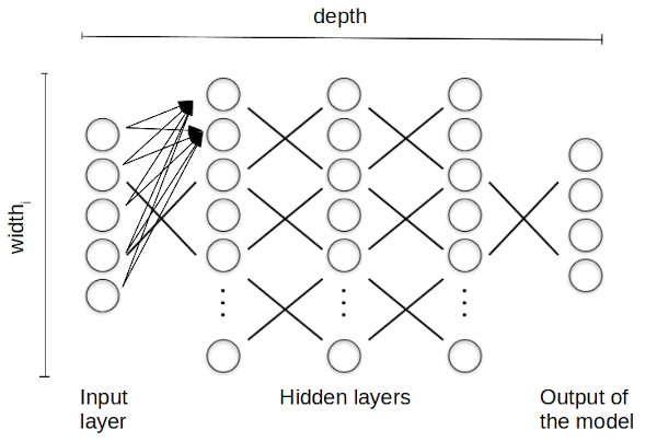
In this layerwise computation, each unit in a particular layer takes input from all the preceding layer units and it has its own parameters that are adjusted to perform the overall computation. The training of the network consists in retrieving the coefficients that minimise a loss function between the output of the model and the known data. In particular, a deep (feedforward) neural network refers to a neural network that contains not only the input and output layers, but also (a variable number of) hidden layers in between.

Neural networks accept only numerical inputs. We hence need to convert all categorical data in numerical units. A common approach is to use the so-called "one-hot-encoding" where the catagorical values are converted into indicator variables (0/1), one for each possible value. This can be done in BetaML using the OneHotEncoder function:

seasonDummies  = fit!(OneHotEncoder(),data.season)
weatherDummies = fit!(OneHotEncoder(),data.weathersit)
wdayDummies    = fit!(OneHotEncoder(),data.weekday .+ 1)


# We compose the feature matrix with the new dimensions obtained from the onehotencoder functions
x = hcat(Matrix{Float64}(data[:,[:instant,:yr,:mnth,:holiday,:workingday,:temp,:atemp,:hum,:windspeed]]),
         seasonDummies,
         weatherDummies,
         wdayDummies)
y = data[:,16];

As we did for decision trees/ random forests, we split the data in training, validation and testing sets

((xtrain,xtest),(ytrain,ytest)) = partition([x,y],[0.75,1-0.75],shuffle=false)
(ntrain, ntest) = size.([ytrain,ytest],1)

2-element Vector{Int64}:
 548
 183

An other common operation with neural networks is to scale the feature vectors (X) and the labels (Y). The BetaML Scaler model, by default, scales the data such that each dimension has mean 0 and variance 1.

Note that we can provide the Scaler` model with different scale factors or specify the columns that shoudn't be scaled (e.g. those resulting from the one-hot encoding). Finally we can reverse the scaling (this is useful to retrieve the unscaled features from a model trained with scaled ones).

cols_nottoscale = [2;4;5;10:23]
xsm             = Scaler(skip=cols_nottoscale)
xtrain_scaled   = fit!(xsm,xtrain)
xtest_scaled    = predict(xsm,xtest)
ytrain_scaled   = ytrain ./ 1000 # We just divide Y by 1000, as using full scaling of Y we may get negative demand.
ytest_scaled    = ytest ./ 1000
D               = size(xtrain,2)

We can now build our feed-forward neaural network. We create three layers, the first layers will always have a input size equal to the dimensions of our data (the number of columns), and the output layer, for a simple regression where the predictions are scalars, it will always be one. We will tune the size of the middle layer size.

There are already several kind of layers available (and you can build your own kind by defining a new struct and implementing a few functions. See the Nn module documentation for details). Here we use only dense layers, those found in typycal feed-fordward neural networks.

For each layer, on top of its size (in "neurons") we can specify an activation function. Here we use the relu for the terminal layer (this will guarantee that our predictions are always positive) and identity for the hidden layer. Again, consult the Nn module documentation for other activation layers already defined, or use any function of your choice.

Initial weight parameters can also be specified if needed. By default DenseLayer use the so-called Xavier initialisation.

Let's hence build our candidate neural network structures, choosing between 5 and 10 nodes in the hidden layers:

candidate_structures = [
        [DenseLayer(D,k,f=relu,df=drelu,rng=copy(AFIXEDRNG)),     # Activation function is ReLU, it's derivative is drelu
         DenseLayer(k,k,f=identity,df=identity,rng=copy(AFIXEDRNG)), # This is the hidden layer we vant to test various sizes
         DenseLayer(k,1,f=relu,df=didentity,rng=copy(AFIXEDRNG))] for k in 5:2:10]

3-element Vector{Vector{DenseLayer{TF, TDF, Float64} where {TF<:Function, TDF<:Union{Nothing, Function}}}}:
 [DenseLayer{typeof(relu), typeof(drelu), Float64}([-0.29531296438620935 -0.015470333744021791 … 0.22698611148327613 0.2904274420874035; -0.12268047123900877 0.24439218426433357 … 0.36149589819305356 0.25651053821356756; … ; -0.4233492331828929 0.013929076127145168 … 0.12727781451876424 -0.3220056051786648; -0.05740921476706312 -0.004590477627889222 … 0.33006927322971974 -0.3229902182657409], [-0.16275699771952834, 0.2715510654801558, -0.3773528046642076, -0.15805165866556825, -0.45768862798217264], BetaML.Utils.relu, BetaML.Utils.drelu), DenseLayer{typeof(identity), typeof(identity), Float64}([-0.49415310523844497 -0.025886819681528617 … 0.09224620317870791 -0.2298725180847525; -0.20528369264408397 0.40894634274263597 … 0.01065168104625569 0.04243100148415224; … ; -0.7083987613359595 0.023307802404264888 … -0.3619336136169306 -0.4825559053138102; -0.09606399030062296 -0.0076813382679077336 … -0.3824319138128976 0.21378287379211514], [-0.11178452751598777, -0.2115472973462721, 0.12029035453379433, -0.06939594013486328, -0.5177091839997635], identity, identity), DenseLayer{typeof(relu), typeof(didentity), Float64}([-0.6379489156883928 -0.2650201076194998 … -0.9145388683760447 -0.12401807820151456], [-0.033419740504278206], BetaML.Utils.relu, BetaML.Utils.didentity)]
 [DenseLayer{typeof(relu), typeof(drelu), Float64}([-0.28529942833030564 0.379669223140765 … 0.28591139889714334 0.2606243753947177; -0.11852059520830227 0.01345676599232093 … -0.29706242768791313 0.23712909181525033; … ; -0.014945762311593835 0.3365486213316541 … 0.38625836286183857 -0.3815582599599021; 0.2361052810665739 0.39732182872463784 … -0.16904473533198983 0.4058193222986791], [-0.2941231824618411, 0.22676070936994097, 0.36548939215338183, 0.2223280912744705, 0.14878832348318172, 0.14237054395672044, 0.12194600561371483], BetaML.Utils.relu, BetaML.Utils.drelu), DenseLayer{typeof(identity), typeof(identity), Float64}([-0.41763559937958017 0.5557788338390783 … 0.4559073525474535 -0.36261818505175825; -0.17349638626452868 0.01969868837033595 … 0.14788575447060037 0.12932806923843965; … ; -0.021878355795233784 0.4926567361624343 … 0.053199618796913706 -0.06119821157571559; 0.34562274152460515 0.5816196024546281 … 0.41959953754300483 -0.0549751039594103], [0.4400179121658523, 0.24489574852922413, -0.19121243996167125, -0.4563330828793923, 0.2666684007070268, 0.37420770408480153, 0.06760655291977202], identity, identity), DenseLayer{typeof(relu), typeof(didentity), Float64}([-0.5524799673028851 -0.22951414571217266 … -0.028942344264588638 0.4572159107612309], [0.7352262891458451], BetaML.Utils.relu, BetaML.Utils.didentity)]
 [DenseLayer{typeof(relu), typeof(drelu), Float64}([-0.27623998365144253 -0.0042939986313030865 … 0.03954785061772442 -0.08082404539953181; -0.11475707285608633 0.17436554863663706 … -0.05561917436604025 -0.21782018027072575; … ; 0.36761314457292255 0.005954470723518457 … -0.3837383360631904 0.3467117277857586; 0.013029457645517328 0.12646036547257528 … 0.22589917353995687 -0.05220438901739144], [0.38096922973233555, -0.17198944163464452, 0.3231333343145583, 0.07247817545621887, 0.2610547851810732, 0.32440076793779044, -0.36628335178017296, -0.09725122313424439, 0.005944201402634575], BetaML.Utils.relu, BetaML.Utils.drelu), DenseLayer{typeof(identity), typeof(identity), Float64}([-0.36831997820192347 -0.005725331508404152 … -0.3958593058455864 -0.009396020856098364; -0.15300943047478177 0.23248739818218278 … -0.5034837638317298 -0.42198614060305667; … ; 0.49015085943056347 0.007939294298024535 … -0.08579127354734356 0.12048358271778759; 0.01737261019402303 0.16861382063010033 … 0.4925234679180297 -0.18459818635959535], [-0.4747622464385455, -0.2650918386962326, -0.2416897178346205, -0.4434088787999071, 0.40076564807210224, 0.36252051789995865, -0.5078601012084061, -0.09079195063298717, 0.2076336496753396], identity, identity), DenseLayer{typeof(relu), typeof(didentity), Float64}([-0.49415310523844497 -0.20528369264408397 … 0.6576063845500103 0.023307802404264888], [-0.0076813382679077336], BetaML.Utils.relu, BetaML.Utils.didentity)]

Note that specify the derivatives of the activation functions (and of the loss function that we'll see in a moment) it totally optional, as without them BetaML will use [Zygote.jl](https://github.com/FluxML/Zygote.jl for automatic differentiation.

We do also set a few other parameters as "turnable": the number of "epochs" to train the model (the number of iterations trough the whole dataset), the sample size at each batch and the optimisation algorithm to use. Several optimisation algorithms are indeed available, and each accepts different parameters, like the learning rate for the Stochastic Gradient Descent algorithm (SGD, used by default) or the exponential decay rates for the moments estimates for the ADAM algorithm (that we use here, with the default parameters).

The hyperparameter ranges will then look as follow:

hpranges = Dict("layers"     => candidate_structures,
                "epochs"     => rand(copy(AFIXEDRNG),DiscreteUniform(50,100),3), # 3 values sampled at random between 50 and 100
                "batch_size" => [4,8,16],
                "opt_alg"    => [SGD(λ=2),SGD(λ=1),SGD(λ=3),ADAM(λ=0.5),ADAM(λ=1),ADAM(λ=0.25)])

Dict{String, Vector{T} where T} with 4 entries:
  "epochs"     => [93, 64, 81]
  "batch_size" => [4, 8, 16]
  "layers"     => Vector{DenseLayer{TF, TDF, Float64} where {TF<:Function, TDF<…
  "opt_alg"    => BetaML.Nn.OptimisationAlgorithm[SGD(#110, 2.0), SGD(#110, 1.0…

Finally we can build "neural network" NeuralNetworkEstimator model where we "chain" the layers together and we assign a final loss function (again, you can provide your own loss function, if those available in BetaML don't suit your needs):

nnm = NeuralNetworkEstimator(loss=squared_cost, descr="Bike sharing regression model", tunemethod=SuccessiveHalvingSearch(hpranges = hpranges), autotune=true,rng=copy(AFIXEDRNG)) # Build the NN model and use the squared cost (aka MSE) as error function by default

NeuralNetworkEstimator - A Feed-forward neural network (unfitted)

We can now fit and autotune the model:

ŷtrain_scaled = fit!(nnm,xtrain_scaled,ytrain_scaled)

548-element Vector{Float64}:
 1.6276179640617505
 1.6262044395781077
 2.0761172765791973
 1.8405431771565297
 1.9356124405265427
 1.5636071679418582
 1.9302085633254302
 2.097415254682476
 2.173954358117641
 2.0608896521431066
 ⋮
 6.4017498230849395
 6.136690161454252
 5.853918032156246
 5.881135603594055
 6.001419626157912
 6.1567869140403895
 6.321342640942563
 6.441270272772373
 6.292419392193321

The model training is one order of magnitude slower than random forests, altought the memory requirement is approximatly the same.

To obtain the neural network predictions we apply the function predict to the feature matrix X for which we want to generate previsions, and then we rescale y. Normally we would apply here the inverse_predict function, but as we simple divided by 1000, we multiply ŷ by the same amount:

ŷtrain = ŷtrain_scaled .* 1000
ŷtest  = predict(nnm,xtest_scaled) .* 1000

183-element Vector{Float64}:
 6071.248677131902
 6162.579566245744
 5866.734380139832
 6329.305353565081
 6378.723890849184
 6793.329501664079
 6494.632970792898
 5484.620719230336
 5603.586480928083
 5978.904009425071
    ⋮
 4627.658649482946
 3628.7855320105223
 2872.657227464448
 1642.036008995796
 2925.4122022733745
 4233.449896021084
 3614.919209226017
 3534.339396834243
 3449.282959266381

(rme_train, rme_test) = relative_mean_error.([ŷtrain,ŷtest],[ytrain,ytest])
push!(results,["NN",rme_train,rme_test]);

The error is much lower. Let's plot our predictions:

Again, we can start by plotting the estimated vs the observed value:

scatter(ytrain,ŷtrain,xlabel="daily rides",ylabel="est. daily rides",label=nothing,title="Est vs. obs in training period (NN)")

scatter(ytest,ŷtest,xlabel="daily rides",ylabel="est. daily rides",label=nothing,title="Est vs. obs in testing period (NN)")

We now plot across the time dimension, first plotting the whole period (2 years):

ŷtrainfull = vcat(ŷtrain,fill(missing,ntest))
ŷtestfull  = vcat(fill(missing,ntrain), ŷtest)
plot(data[:,:dteday],[data[:,:cnt] ŷtrainfull ŷtestfull], label=["obs" "train" "test"], legend=:topleft, ylabel="daily rides", title="Daily bike sharing demand observed/estimated across the\n whole 2-years period  (NN)")

...and then focusing on the testing data

stc  = 620
endc = size(x,1)
plot(data[stc:endc,:dteday],[data[stc:endc,:cnt] ŷtestfull[stc:endc]], label=["obs" "val" "test"], legend=:bottomleft, ylabel="Daily rides", title="Focus on the testing period (NN)")

Comparison with Flux.jl

We now apply the same Neural Network model using the Flux framework, a dedicated neural network library, reusing the optimal parameters that we did learn from tuning NeuralNetworkEstimator:

hp_opt         = hyperparameters(nnm)
opt_size       = size(hp_opt.layers[1])[2][1]
opt_batch_size = hp_opt.batch_size
opt_epochs     = hp_opt.epochs

We fix the default random number generator so that the Flux example gives a reproducible output

Random.seed!(seed)

MersenneTwister(123)

We define the Flux neural network model and load it with data...

l1         = Flux.Dense(D,opt_size,Flux.relu)
l2         = Flux.Dense(opt_size,opt_size,identity)
l3         = Flux.Dense(opt_size,1,Flux.relu)
Flux_nn    = Flux.Chain(l1,l2,l3)
fluxloss(x, y) = Flux.mse(Flux_nn(x), y)
ps         = Flux.params(Flux_nn)
nndata     = Flux.Data.DataLoader((xtrain_scaled', ytrain_scaled'), batchsize=opt_batch_size,shuffle=true)

137-element DataLoader(::Tuple{LinearAlgebra.Adjoint{Float64, Matrix{Float64}}, LinearAlgebra.Adjoint{Float64, Vector{Float64}}}, shuffle=true, batchsize=4)
  with first element:
  (23×4 Matrix{Float64}, 1×4 adjoint(::Vector{Float64}) with eltype Float64,)

We do the training of the Flux model...

[Flux.train!(fluxloss, ps, nndata, Flux.ADAM(0.001, (0.9, 0.8))) for i in 1:opt_epochs]

93-element Vector{Nothing}:
 nothing
 nothing
 nothing
 nothing
 nothing
 nothing
 nothing
 nothing
 nothing
 nothing
 ⋮
 nothing
 nothing
 nothing
 nothing
 nothing
 nothing
 nothing
 nothing
 nothing

We obtain the predicitons...

ŷtrainf = @pipe Flux_nn(xtrain_scaled')' .* 1000;
ŷtestf  = @pipe Flux_nn(xtest_scaled')'  .* 1000;

┌ Warning: Layer with Float32 parameters got Float64 input.
│   The input will be converted, but any earlier layers may be very slow.
│   layer = Dense(23 => 9, relu)  # 216 parameters
│   summary(x) = "23×548 adjoint(::Matrix{Float64}) with eltype Float64"
└ @ Flux ~/.julia/packages/Flux/n3cOc/src/layers/stateless.jl:60
┌ Warning: Layer with Float32 parameters got Float64 input.
│   The input will be converted, but any earlier layers may be very slow.
│   layer = Dense(23 => 9, relu)  # 216 parameters
│   summary(x) = "23×183 adjoint(::Matrix{Float64}) with eltype Float64"
└ @ Flux ~/.julia/packages/Flux/n3cOc/src/layers/stateless.jl:60

..and we compute the mean relative errors..

(rme_train, rme_test) = relative_mean_error.([ŷtrainf,ŷtestf],[ytrain,ytest])
push!(results,["NN (Flux.jl)",rme_train,rme_test]);

.. finding an error not significantly different than the one obtained from BetaML.Nn.

Plots:

scatter(ytrain,ŷtrainf,xlabel="daily rides",ylabel="est. daily rides",label=nothing,title="Est vs. obs in training period (Flux.NN)")

scatter(ytest,ŷtestf,xlabel="daily rides",ylabel="est. daily rides",label=nothing,title="Est vs. obs in testing period (Flux.NN)")

ŷtrainfullf = vcat(ŷtrainf,fill(missing,ntest))
ŷtestfullf  = vcat(fill(missing,ntrain), ŷtestf)
plot(data[:,:dteday],[data[:,:cnt] ŷtrainfullf ŷtestfullf], label=["obs" "train" "test"], legend=:topleft, ylabel="daily rides", title="Daily bike sharing demand observed/estimated across the\n whole 2-years period (Flux.NN)")

stc = 620
endc = size(x,1)
plot(data[stc:endc,:dteday],[data[stc:endc,:cnt] ŷtestfullf[stc:endc]], label=["obs" "val" "test"], legend=:bottomleft, ylabel="Daily rides", title="Focus on the testing period (Flux.NN)")

Conclusions of Neural Network models

If we strive for the most accurate predictions, deep neural networks are usually the best choice. However they are computationally expensive, so with limited resourses we may get better results by fine tuning and running many repetitions of "simpler" decision trees or even random forest models than a large naural network with insufficient hyper-parameter tuning. Also, we shoudl consider that decision trees/random forests are much simpler to work with.

That said, specialised neural network libraries, like Flux, allow to use GPU and specialised hardware letting neural networks to scale with very large datasets.

Still, for small and medium datasets, BetaML provides simpler yet customisable solutions that are accurate and fast.

GMM-based regressors

BetaML 0.8 introduces new regression algorithms based on Gaussian Mixture Model. Specifically, there are two variants available, GaussianMixtureRegressor2 and GaussianMixtureRegressor, and this example uses GaussianMixtureRegressor As for neural networks, they work on numerical data only, so we reuse the datasets we prepared for the neural networks.

As usual we first define the model.

m = GaussianMixtureRegressor(rng=copy(AFIXEDRNG),verbosity=NONE)

GaussianMixtureRegressor - A regressor based on Generative Mixture Model (unfitted)

Info

We disabled autotune here, as this code is run by GitHub continuous_integration servers on each code update, and GitHub servers seem to have some strange problem with it, taking almost 4 hours instead of a few seconds on my machine.

We then fit the model to the training data..

ŷtrainGMM_unscaled = fit!(m,xtrain_scaled,ytrain_scaled)

548×1 Matrix{Float64}:
 2.05456959514988
 2.0545695951498795
 2.0545695951498795
 2.0545695951498795
 2.0545695951498795
 2.0545695951498795
 2.0545695951498795
 2.0545695951498795
 2.0545695951498795
 2.0545695951498795
 ⋮
 5.525359181472882
 5.525359181472882
 5.525359181472882
 5.525359181472882
 5.525359181472882
 5.525359181472882
 5.525359181472882
 5.525359181472882
 5.525359181472882

And we predict...

ŷtrainGMM = ŷtrainGMM_unscaled .* 1000;
ŷtestGMM  = predict(m,xtest_scaled)  .* 1000;

(rme_train, rme_test) = relative_mean_error.([ŷtrainGMM,ŷtestGMM],[ytrain,ytest])
push!(results,["GMM",rme_train,rme_test]);

Summary

This is the summary of the results (train and test relative mean error) we had trying to predict the daily bike sharing demand, given weather and calendar information:

println(results)

6×3 DataFrame
 Row │ model                 train_rme  test_rme
     │ String                Float64    Float64
─────┼───────────────────────────────────────────
   1 │ DT                    0.0213416  0.172881
   2 │ RF                    0.0469041  0.166364
   3 │ RF (DecisionTree.jl)  0.0987308  0.286927
   4 │ NN                    0.149393   0.166221
   5 │ NN (Flux.jl)          0.08599    0.172753
   6 │ GMM                   0.216144   0.26681

You may ask how stable are these results? How much do they depend from the specific RNG seed ? We re-evaluated a couple of times the whole script but changing random seeds (to 1000 and 10000):

Model	Train rme1	Test rme1	Train rme2	Test rme2	Train rme3	Test rme3
DT	0.1366960	0.154720	0.0233044	0.249329	0.0621571	0.161657
RF	0.0421267	0.180186	0.0535776	0.136920	0.0386144	0.141606
RF (DecisionTree.jl)	0.0230439	0.235823	0.0801040	0.243822	0.0168764	0.219011
NN	0.1604000	0.169952	0.1091330	0.121496	0.1481440	0.150458
NN (Flux.jl)	0.0931161	0.166228	0.0920796	0.167047	0.0907810	0.122469
GaussianMixtureRegressor*	0.1432800	0.293891	0.1380340	0.295470	0.1477570	0.284567

GMM is a deterministic model, the variations are due to the different random sampling in choosing the best hyperparameters

Neural networks can be more precise than random forests models, but are more computationally expensive (and tricky to set up). When we compare BetaML with the algorithm-specific leading packages, we found similar results in terms of accuracy, but often the leading packages are better optimised and run more efficiently (but sometimes at the cost of being less versatile). GMM_based regressors are very computationally cheap and a good compromise if accuracy can be traded off for performances.

View this file on Github.

This page was generated using Literate.jl.