Videos related to this segment (click the title to watch)

02 JULIA2 - 2A: Plotting (15:18)

02 JULIA2 - 2B: Probability distributions and data fitting (11:55)

02 JULIA2 - 2C: Constrained optimisation, the transport problem (24:59)

02 JULIA2 - 2D: Nonlinear constrained optimisation, the optimal portfolio allocation (16:4)

0202 - Miscellaneous topics

Some stuff to set-up the environment..

julia> cd(@__DIR__)
julia> using Pkg
julia> Pkg.activate(".")
       # If using a Julia version different than 1.10 please uncomment and run the following line (reproductibility guarantee will hower be lost)
       # Pkg.resolve()
       # Pkg.instantiate() # run this if you didn't in Segment 02.01  Activating project at `~/work/SPMLJ/SPMLJ/buildedDoc/02_-_JULIA2_-_Scientific_programming_with_Julia`
julia> using Random
julia> Random.seed!(123)Random.TaskLocalRNG()

Plotting

Within the many possible packages to plot in Julia we use here the Plots package that allows at run time to choose the plot's backend. The defauld backend is gr (that, if you want to go back to it after you choosen another backend, you can activate with gr()). Other common backends are the Python MatplotLib (pyplot(), requiring package PyPlot) and Plotly (plotlyjs() from package PlotlyJS). Actually we use StatsPlots that just adds a set of convenient functionalities (in plots terminology called "recipes") on top of Plots.

julia> using StatsPlots # no need to `using Plots` as `Plots` elements are reexported by StatsPlots

The basic idea is that we can draw different "graphical elements" in a Plot figure. The plot(.) function will first create a new figure, while plot!(.) will modify an existing plot (by drawing new elements on it, such as a new serie) taking the "current" plot as default if no plot object is passed as first argument.

Plotting functions

Let's start plotting a function. The FIRST TIME you invoke plot will take a while. This is the famous "time to first plot" problem due to the JIT compilation, but it will materialize only on the first plotting in a working session

julia> plot(cos) # default [-5,+5] rangePlot{Plots.GRBackend() n=1}

julia> plot!(x->x^2, -2,2 ) # more explicit, with rangesPlot{Plots.GRBackend() n=2}

julia> plot!(x->max(x,2), label="max function", linestyle=:dot, color=:black, title="Chart title", xlabel= "X axis", ylabel="Y axis", legend=:topleft) # a bit of designPlot{Plots.GRBackend() n=3}

julia> plot!(twinx(),x->20x,colour=RGB(20/255,120/255,13/255)) # secondary axisPlot{Plots.GRBackend() n=4}

Plotting data

julia> using DataFrames
julia> x = 11:1511:15
julia> data = DataFrame(a=[4,8,6,6,3], b=[2,4,5,8,6], c=[20,40,15,5,30])5×3 DataFrame
 Row │ a      b      c
     │ Int64  Int64  Int64
─────┼─────────────────────
   1 │     4      2     20
   2 │     8      4     40
   3 │     6      5     15
   4 │     6      8      5
   5 │     3      6     30
julia> plot(x, Matrix(data)) # x, series (in column)Plot{Plots.GRBackend() n=3}

julia> @df data plot(x, :a, seriestype=:bar, legend=:topleft)Plot{Plots.GRBackend() n=1}

julia> plot!(x, data.b, seriestype=:line)Plot{Plots.GRBackend() n=2}

julia> scatter!(twinx(), x, data.c) # alias for `plot!(..., seriestype=:scatter)`Plot{Plots.GRBackend() n=3}

Layouts with multiple plots

julia> l = @layout [a ; b c] # a,b,c, here are just placeholders, not related with the df column names..2×1 Matrix{Any}:
 (label = :a, blank = false)
 Any[(label = :b, blank = false) (label = :c, blank = false)]
julia> p1 = plot(x, data.a)Plot{Plots.GRBackend() n=1}
julia> p2 = scatter(x, data.b)Plot{Plots.GRBackend() n=1}
julia> p3 = plot(x, data.c)Plot{Plots.GRBackend() n=1}
julia> plot(p1, p2, p3, layout = l)Plot{Plots.GRBackend() n=3}

Saving the plot..

julia> savefig("myplot.png")"/home/runner/work/SPMLJ/SPMLJ/buildedDoc/02_-_JULIA2_-_Scientific_programming_with_Julia/myplot.png"
julia> savefig("myplot.pdf")"/home/runner/work/SPMLJ/SPMLJ/buildedDoc/02_-_JULIA2_-_Scientific_programming_with_Julia/myplot.pdf"
julia> savefig("myplot.svg")"/home/runner/work/SPMLJ/SPMLJ/buildedDoc/02_-_JULIA2_-_Scientific_programming_with_Julia/myplot.svg"

Probabilistic analysis

Julia has a very elegant package to deal with probability analysis, the Distributions package.

julia> using Distributions

The idea is that we first create a Distribution object, of the distribution family and with the parameter required, and then we operate on it, for example to sample or to retrieve a quantile. The following table gives the distribution constructors for some of the most common distributions:

Discrete distr.	Constructor	Continuous distr.	Constructor
Discrete uniform	`DiscreteUniform(lRange,uRange)`	Uniform	`Uniform(lRange,uRange)`
Bernoulli	`Bernoulli(p)`	Exponential	`Exponential(rate)`
Binomial	`Binomial(n,p)`	Laplace	`Laplace(loc, scale)`
Categorical	`Categorical(ps)`	Normal	`Normal(μ,σ)`
Multinomial	`Multinomial(n, ps)`	Erlang	`Erlang(n,rate)`
Geometric	`Geometric(p)`	Cauchy	`Cauchy(μ, σ)`
Hypergeometric	`Hypergeometric(nS, nF, nTrials)`	Chisq	`Chisq(df)`
Poisson	`Poisson(rate)`	T Dist	`TDist(df)`
Negative Binomial	`NegativeBinomial(nSucc,p)`	F Dist	`FDist(df1, df2)`
		Beta Dist	`Beta(shapeα,shapeβ)`
		Gamma Dist	`Gamma(shapeα,1/rateβ)`

julia> d = Normal(10,3) # note that the parameter is the standard deviation, not the varianceDistributions.Normal{Float64}(μ=10.0, σ=3.0)
julia> mean(d)10.0
julia> var(d)9.0
julia> median(d)10.0
julia> quantile(d,0.9)13.844654696633802
julia> cdf(d,13.844)0.8999616952550467
julia> pdf(d,0)0.0005140929987637017
julia> rand(d,3,4,2)3×4×2 Array{Float64, 3}:
[:, :, 1] =
 12.4249    8.74902   8.73469   9.64803
  6.63378  10.8628    5.93323  13.6578
  6.68609  10.6895   10.2084   10.8787

[:, :, 2] =
  9.90656   7.32977   9.04339  12.2951
 10.9475   12.5627    8.98764  10.5408
  3.51286  11.0253   16.0243   16.0867
julia> sample = rand(d,1000);
julia> density(sample)Plot{Plots.GRBackend() n=1}

julia> plot!(d)Plot{Plots.GRBackend() n=2}

julia> fit(Normal, sample) # using MLEDistributions.Normal{Float64}(μ=10.130363752262184, σ=3.0557996927248805)

For a quick overview on the various distributions available, the main methods that apply to them and a comparision with equivvalent R and Python libraries, you can see this cheatsheet: https://github.com/sylvaticus/commonDistributionsInJuliaPythonR

Curve fitting

LsqFit is a very flexible data fitting package for linear and nonlinear arbitrary functions (using least squares). Let's use it to fit a logistic growth curve (Verhulst model) of volumes for a forest stand.

julia> using LsqFit
julia> data = DataFrame(
           age = 20:5:90,
           vol = [64,112,170,231,293,352,408,459,505,546,582,613,640,663,683]
       ) # Scots Pine, data from the UK Forestry Commission https://web.archive.org/web/20170119072737/http://forestry.gov.uk/pdf/FCBK048.pdf/$FILE/FCBK048.pdf15×2 DataFrame
 Row │ age    vol
     │ Int64  Int64
─────┼──────────────
   1 │    20     64
   2 │    25    112
   3 │    30    170
   4 │    35    231
   5 │    40    293
   6 │    45    352
   7 │    50    408
   8 │    55    459
   9 │    60    505
  10 │    65    546
  11 │    70    582
  12 │    75    613
  13 │    80    640
  14 │    85    663
  15 │    90    683
julia> plot(data.vol)Plot{Plots.GRBackend() n=1}

julia> logisticModel(age,parameters) = parameters[1]/(1+exp(-parameters[2] * (age-parameters[3]) ))logisticModel (generic function with 1 method)
julia> logisticModelVec(age,parameters) = logisticModel.(age,Ref(parameters))logisticModelVec (generic function with 1 method)
julia> initialParameters = [1000,0.02,50] #max growth; growth rate, mid age3-element Vector{Float64}:
 1000.0
    0.02
   50.0
julia> fitobject         = curve_fit(logisticModelVec, data.age, data.vol, initialParameters)LsqFit.LsqFitResult{Vector{Float64}, Vector{Float64}, Matrix{Float64}, Vector{Int64}, Vector{LsqFit.LMState{LsqFit.LevenbergMarquardt}}}([692.5825413198176, 0.07303427530184728, 45.521079747040055], [28.97750654863104, 14.474712045689813, -1.3542656293281539, -11.572229993633243, -15.595058416636618, -12.297282501188477, -5.569946832007304, 2.589144258849501, 9.03778220094398, 12.04852281878334, 11.305933439776368, 7.516649845482561, 0.9186273616159042, -7.113657843007559, -16.307121770578988], [0.13424754596426883 -2054.332191201643 -5.878930833729613; 0.18261319698514056 -2121.443789792599 -7.550192857774018; … ; 0.9470154140969926 1371.9661652874784 -2.538077366652955; 0.9626186605328434 1108.4980035787337 -1.8201509196993966], true, Iter     Function value   Gradient norm
------   --------------   --------------
, Int64[])
julia> fitparams         = fitobject.param3-element Vector{Float64}:
 692.5825413198176
   0.07303427530184728
  45.521079747040055
julia> fitobject.resid15-element Vector{Float64}:
  28.97750654863104
  14.474712045689813
  -1.3542656293281539
 -11.572229993633243
 -15.595058416636618
 -12.297282501188477
  -5.569946832007304
   2.589144258849501
   9.03778220094398
  12.04852281878334
  11.305933439776368
   7.516649845482561
   0.9186273616159042
  -7.113657843007559
 -16.307121770578988
julia> residuals = logisticModelVec(data.age,fitparams) .- data.vol15-element Vector{Float64}:
  28.97750654863104
  14.474712045689813
  -1.3542656293281539
 -11.572229993633243
 -15.595058416636618
 -12.297282501188477
  -5.569946832007304
   2.589144258849501
   9.03778220094398
  12.04852281878334
  11.305933439776368
   7.516649845482561
   0.9186273616159042
  -7.113657843007559
 -16.307121770578988
julia> fitobject.resid == residualstrue
julia> sigma            = stderror(fitobject)3-element Vector{Float64}:
 12.682368775164093
  0.0035444978136088046
  0.7982532437259628
julia> confidence_inter = confidence_interval(fitobject, 0.05) # 5% significance level3-element Vector{Tuple{Float64, Float64}}:
 (664.950033521919, 720.2150491177161)
 (0.06531147799082898, 0.08075707261286558)
 (43.78183533828645, 47.26032415579366)
julia> x = 0:maximum(data.age)*1.50.0:1.0:135.0
julia> plot(x->logisticModel(x,fitparams),0,maximum(x), label= "Fitted vols", legend=:topleft)Plot{Plots.GRBackend() n=1}
julia> plot!(data.age, data.vol, seriestype=:scatter, label = "Obs vols")Plot{Plots.GRBackend() n=2}
julia> plot!(data.age, residuals, seriestype=:bar, label = "Residuals")Plot{Plots.GRBackend() n=3}

Constrained optimisation

JuMP is the leading library to express complex optimisation problems in a clear, mathematical friendly syntax, compute the information required by the solver engines to solve the optimisation problem, pass the problem to the aforementioned solver engines and retrieve the solutions.

JuMP has the same flexibility and expressivity of dedicated algeabric modelling languages as GAMS or AMPL but with the advantage of being a library within a much more general programming language, with larger community, development tools, language constructs and possibility to interface the specific "optimisation component" of a model with the rest of the model.

We will see how to specify the variables, the constraints and the objective function of an optimisation model, how to "solve" it and how to retrieve the optimal values

A linear example: the classical "transport" problem

Obj: minimise transport costs $c$ from several plants $p$ to several markets $m$ under the contraint to satisfy the demand $d_m$ at each market while respecting the production capacity $c_p$ of each plant: $min_{x_{p,m}} \sum_p \sum_m c_{p,m} * x_{p,m}$ subject to: $\sum_m x_{p,m} \leq d_m$ $\sum_p x_{p,m} \geq c_m$

julia> using  JuMP, GLPK, DataFrames, CSV

"Sets" and exogenous parameters definition

index sets

julia> orig = ["Epinal", "Bordeaux", "Grenoble"] # plant/sawmills origin of timber3-element Vector{String}:
 "Epinal"
 "Bordeaux"
 "Grenoble"
julia> dest = ["Paris", "Lyon", "Nantes", "Tulouse", "Lille", "Marseille", "Strasbourg"] # markets7-element Vector{String}:
 "Paris"
 "Lyon"
 "Nantes"
 "Tulouse"
 "Lille"
 "Marseille"
 "Strasbourg"
julia> prod = ["Fuelwood", "Sawnwood", "Pannels"]3-element Vector{String}:
 "Fuelwood"
 "Sawnwood"
 "Pannels"

Read input data into DataFrames and then into Dictionaries with 2D or 3D tuples of index sets as keys

supply(prod, orig) amounts available at origins

julia> supplytable = CSV.read(IOBuffer("""
       prod     Epinal Bordeaux Grenoble
       Fuelwood 400    700      800
       Sawnwood 800    1600     1800
       Pannels  200    300      300
       """), DataFrame, delim=" ", ignorerepeated=true,copycols=true)3×4 DataFrame
 Row │ prod      Epinal  Bordeaux  Grenoble
     │ String15  Int64   Int64     Int64
─────┼──────────────────────────────────────
   1 │ Fuelwood     400       700       800
   2 │ Sawnwood     800      1600      1800
   3 │ Pannels      200       300       300
julia> supply = Dict( (r[:prod],o) => r[Symbol(o)] for r in eachrow(supplytable), o in orig)Dict{Tuple{InlineStrings.String15, String}, Int64} with 9 entries:
  ("Sawnwood", "Bordeaux") => 1600
  ("Sawnwood", "Epinal")   => 800
  ("Pannels", "Epinal")    => 200
  ("Pannels", "Bordeaux")  => 300
  ("Pannels", "Grenoble")  => 300
  ("Fuelwood", "Epinal")   => 400
  ("Fuelwood", "Bordeaux") => 700
  ("Fuelwood", "Grenoble") => 800
  ("Sawnwood", "Grenoble") => 1800

demand(prod, dest) amounts required at destinations

julia> demandtable = CSV.read(IOBuffer("""
       prod      Paris Lyon Nantes Tulouse Lille Marseille Strasbourg
       Fuelwood  300   300  100    75      650   225       250
       Sawnwood  500   750  400    250     950   850       500
       Pannels   100   100  0      50      200   100       250
       """), DataFrame, delim=" ", ignorerepeated=true,copycols=true)3×8 DataFrame
 Row │ prod      Paris  Lyon   Nantes  Tulouse  Lille  Marseille  Strasbourg
     │ String15  Int64  Int64  Int64   Int64    Int64  Int64      Int64
─────┼───────────────────────────────────────────────────────────────────────
   1 │ Fuelwood    300    300     100       75    650        225         250
   2 │ Sawnwood    500    750     400      250    950        850         500
   3 │ Pannels     100    100       0       50    200        100         250
julia> demand = Dict( (r[:prod],d) => r[Symbol(d)] for r in eachrow(demandtable), d in dest)Dict{Tuple{InlineStrings.String15, String}, Int64} with 21 entries:
  ("Fuelwood", "Paris")      => 300
  ("Pannels", "Paris")       => 100
  ("Pannels", "Lyon")        => 100
  ("Sawnwood", "Tulouse")    => 250
  ("Fuelwood", "Tulouse")    => 75
  ("Fuelwood", "Nantes")     => 100
  ("Sawnwood", "Lyon")       => 750
  ("Pannels", "Tulouse")     => 50
  ("Fuelwood", "Lille")      => 650
  ("Pannels", "Nantes")      => 0
  ("Sawnwood", "Lille")      => 950
  ("Pannels", "Marseille")   => 100
  ("Fuelwood", "Lyon")       => 300
  ("Fuelwood", "Strasbourg") => 250
  ("Sawnwood", "Paris")      => 500
  ("Sawnwood", "Nantes")     => 400
  ("Fuelwood", "Marseille")  => 225
  ("Pannels", "Strasbourg")  => 250
  ("Sawnwood", "Strasbourg") => 500
  ⋮                          => ⋮

limit(orig, dest) of total units from any origin to destination

julia> defaultlimit = 625.0625.0
julia> limit = Dict((o,d) => defaultlimit for o in orig, d in dest)Dict{Tuple{String, String}, Float64} with 21 entries:
  ("Bordeaux", "Lyon")       => 625.0
  ("Epinal", "Lille")        => 625.0
  ("Bordeaux", "Marseille")  => 625.0
  ("Epinal", "Marseille")    => 625.0
  ("Grenoble", "Paris")      => 625.0
  ("Grenoble", "Marseille")  => 625.0
  ("Bordeaux", "Lille")      => 625.0
  ("Grenoble", "Tulouse")    => 625.0
  ("Epinal", "Strasbourg")   => 625.0
  ("Epinal", "Tulouse")      => 625.0
  ("Bordeaux", "Nantes")     => 625.0
  ("Grenoble", "Lille")      => 625.0
  ("Grenoble", "Nantes")     => 625.0
  ("Grenoble", "Lyon")       => 625.0
  ("Bordeaux", "Strasbourg") => 625.0
  ("Grenoble", "Strasbourg") => 625.0
  ("Epinal", "Nantes")       => 625.0
  ("Epinal", "Paris")        => 625.0
  ("Bordeaux", "Paris")      => 625.0
  ⋮                          => ⋮

cost(prod, orig, dest) Shipment cost per unit

julia> costtable = CSV.read(IOBuffer("""
       prod     orig     Paris Lyon Nantes Tulouse Lille Marseille Strasbourg
       Fuelwood Epinal   30    10   8      10      11    71        6
       Fuelwood Bordeaux 22    7    10     7       21    82        13
       Fuelwood Grenoble 19    11   12     10      25    83        15
       
       Sawnwood Epinal   39    14   11     14      16    82        8
       Sawnwood Bordeaux 27    9    12     9       26    95        17
       Sawnwood Grenoble 24    14   17     13      28    99        20
       
       Pannels  Epinal   41    15   12     16      17    86        8
       Pannels  Bordeaux 29    9    13     9       28    99        18
       Pannels  Grenoble 26    14   17     13      31    104       20
       """), DataFrame, delim=" ", ignorerepeated=true,copycols=true)9×9 DataFrame
 Row │ prod      orig      Paris  Lyon   Nantes  Tulouse  Lille  Marseille  St ⋯
     │ String15  String15  Int64  Int64  Int64   Int64    Int64  Int64      In ⋯
─────┼──────────────────────────────────────────────────────────────────────────
   1 │ Fuelwood  Epinal       30     10       8       10     11         71     ⋯
   2 │ Fuelwood  Bordeaux     22      7      10        7     21         82
   3 │ Fuelwood  Grenoble     19     11      12       10     25         83
   4 │ Sawnwood  Epinal       39     14      11       14     16         82
   5 │ Sawnwood  Bordeaux     27      9      12        9     26         95     ⋯
   6 │ Sawnwood  Grenoble     24     14      17       13     28         99
   7 │ Pannels   Epinal       41     15      12       16     17         86
   8 │ Pannels   Bordeaux     29      9      13        9     28         99
   9 │ Pannels   Grenoble     26     14      17       13     31        104     ⋯
                                                                1 column omitted
julia> cost = Dict( (r[:prod],r[:orig],d) => r[Symbol(d)] for r in eachrow(costtable), d in dest)Dict{Tuple{InlineStrings.String15, InlineStrings.String15, String}, Int64} with 63 entries:
  ("Sawnwood", "Epinal", "Lille")        => 16
  ("Sawnwood", "Epinal", "Paris")        => 39
  ("Sawnwood", "Bordeaux", "Lyon")       => 9
  ("Sawnwood", "Epinal", "Lyon")         => 14
  ("Sawnwood", "Bordeaux", "Strasbourg") => 17
  ("Fuelwood", "Bordeaux", "Tulouse")    => 7
  ("Fuelwood", "Bordeaux", "Lille")      => 21
  ("Fuelwood", "Grenoble", "Strasbourg") => 15
  ("Sawnwood", "Grenoble", "Strasbourg") => 20
  ("Fuelwood", "Grenoble", "Lyon")       => 11
  ("Fuelwood", "Bordeaux", "Lyon")       => 7
  ("Sawnwood", "Grenoble", "Lille")      => 28
  ("Pannels", "Bordeaux", "Tulouse")     => 9
  ("Fuelwood", "Grenoble", "Nantes")     => 12
  ("Pannels", "Epinal", "Lyon")          => 15
  ("Sawnwood", "Bordeaux", "Tulouse")    => 9
  ("Pannels", "Bordeaux", "Paris")       => 29
  ("Fuelwood", "Bordeaux", "Paris")      => 22
  ("Sawnwood", "Epinal", "Nantes")       => 11
  ⋮                                      => ⋮

Optimisation model definition

julia> trmodel = Model(GLPK.Optimizer)A JuMP Model
Feasibility problem with:
Variables: 0
Model mode: AUTOMATIC
CachingOptimizer state: EMPTY_OPTIMIZER
Solver name: GLPK
julia> set_optimizer_attribute(trmodel, "msg_lev", GLPK.GLP_MSG_ON)

...

Alternativelly, you can use HiGHS as another popular choice for linear solver engine

Model's endogenous variables definition

julia> @variables trmodel begin
           x[p in prod, o in orig, d in dest] >= 0
       end;

Constraints definition

julia> @constraints trmodel begin
           supply[p in prod, o in orig], # observe supply limit at plant/sawmill origin o
               sum(x[p,o,d] for d in dest) <= supply[p,o]
           demand[p in prod, d in dest], # satisfy demand at market dest d
               sum(x[p,o,d] for o in orig) >= demand[p,d]
           c_total_shipment[o in orig, d in dest],
               sum(x[p,o,d] for p in prod) <= limit[o,d]
       end;

Objective function definition

julia> @objective trmodel Min begin
           sum(cost[p,o,d] * x[p,o,d] for p in prod, o in orig, d in dest)
       end30 x[Fuelwood,Epinal,Paris] + 39 x[Sawnwood,Epinal,Paris] + 41 x[Pannels,Epinal,Paris] + 22 x[Fuelwood,Bordeaux,Paris] + 27 x[Sawnwood,Bordeaux,Paris] + 29 x[Pannels,Bordeaux,Paris] + 19 x[Fuelwood,Grenoble,Paris] + 24 x[Sawnwood,Grenoble,Paris] + 26 x[Pannels,Grenoble,Paris] + 10 x[Fuelwood,Epinal,Lyon] + 14 x[Sawnwood,Epinal,Lyon] + 15 x[Pannels,Epinal,Lyon] + 7 x[Fuelwood,Bordeaux,Lyon] + 9 x[Sawnwood,Bordeaux,Lyon] + 9 x[Pannels,Bordeaux,Lyon] + 11 x[Fuelwood,Grenoble,Lyon] + 14 x[Sawnwood,Grenoble,Lyon] + 14 x[Pannels,Grenoble,Lyon] + 8 x[Fuelwood,Epinal,Nantes] + 11 x[Sawnwood,Epinal,Nantes] + 12 x[Pannels,Epinal,Nantes] + 10 x[Fuelwood,Bordeaux,Nantes] + 12 x[Sawnwood,Bordeaux,Nantes] + 13 x[Pannels,Bordeaux,Nantes] + 12 x[Fuelwood,Grenoble,Nantes] + 17 x[Sawnwood,Grenoble,Nantes] + 17 x[Pannels,Grenoble,Nantes] + 10 x[Fuelwood,Epinal,Tulouse] + 14 x[Sawnwood,Epinal,Tulouse] + 16 x[Pannels,Epinal,Tulouse] + [[...3 terms omitted...]] + 10 x[Fuelwood,Grenoble,Tulouse] + 13 x[Sawnwood,Grenoble,Tulouse] + 13 x[Pannels,Grenoble,Tulouse] + 11 x[Fuelwood,Epinal,Lille] + 16 x[Sawnwood,Epinal,Lille] + 17 x[Pannels,Epinal,Lille] + 21 x[Fuelwood,Bordeaux,Lille] + 26 x[Sawnwood,Bordeaux,Lille] + 28 x[Pannels,Bordeaux,Lille] + 25 x[Fuelwood,Grenoble,Lille] + 28 x[Sawnwood,Grenoble,Lille] + 31 x[Pannels,Grenoble,Lille] + 71 x[Fuelwood,Epinal,Marseille] + 82 x[Sawnwood,Epinal,Marseille] + 86 x[Pannels,Epinal,Marseille] + 82 x[Fuelwood,Bordeaux,Marseille] + 95 x[Sawnwood,Bordeaux,Marseille] + 99 x[Pannels,Bordeaux,Marseille] + 83 x[Fuelwood,Grenoble,Marseille] + 99 x[Sawnwood,Grenoble,Marseille] + 104 x[Pannels,Grenoble,Marseille] + 6 x[Fuelwood,Epinal,Strasbourg] + 8 x[Sawnwood,Epinal,Strasbourg] + 8 x[Pannels,Epinal,Strasbourg] + 13 x[Fuelwood,Bordeaux,Strasbourg] + 17 x[Sawnwood,Bordeaux,Strasbourg] + 18 x[Pannels,Bordeaux,Strasbourg] + 15 x[Fuelwood,Grenoble,Strasbourg] + 20 x[Sawnwood,Grenoble,Strasbourg] + 20 x[Pannels,Grenoble,Strasbourg]

Human-readable visualisation of the model

julia> print(trmodel)Min 30 x[Fuelwood,Epinal,Paris] + 39 x[Sawnwood,Epinal,Paris] + 41 x[Pannels,Epinal,Paris] + 22 x[Fuelwood,Bordeaux,Paris] + 27 x[Sawnwood,Bordeaux,Paris] + 29 x[Pannels,Bordeaux,Paris] + 19 x[Fuelwood,Grenoble,Paris] + 24 x[Sawnwood,Grenoble,Paris] + 26 x[Pannels,Grenoble,Paris] + 10 x[Fuelwood,Epinal,Lyon] + 14 x[Sawnwood,Epinal,Lyon] + 15 x[Pannels,Epinal,Lyon] + 7 x[Fuelwood,Bordeaux,Lyon] + 9 x[Sawnwood,Bordeaux,Lyon] + 9 x[Pannels,Bordeaux,Lyon] + 11 x[Fuelwood,Grenoble,Lyon] + 14 x[Sawnwood,Grenoble,Lyon] + 14 x[Pannels,Grenoble,Lyon] + 8 x[Fuelwood,Epinal,Nantes] + 11 x[Sawnwood,Epinal,Nantes] + 12 x[Pannels,Epinal,Nantes] + 10 x[Fuelwood,Bordeaux,Nantes] + 12 x[Sawnwood,Bordeaux,Nantes] + 13 x[Pannels,Bordeaux,Nantes] + 12 x[Fuelwood,Grenoble,Nantes] + 17 x[Sawnwood,Grenoble,Nantes] + 17 x[Pannels,Grenoble,Nantes] + 10 x[Fuelwood,Epinal,Tulouse] + 14 x[Sawnwood,Epinal,Tulouse] + 16 x[Pannels,Epinal,Tulouse] + [[...3 terms omitted...]] + 10 x[Fuelwood,Grenoble,Tulouse] + 13 x[Sawnwood,Grenoble,Tulouse] + 13 x[Pannels,Grenoble,Tulouse] + 11 x[Fuelwood,Epinal,Lille] + 16 x[Sawnwood,Epinal,Lille] + 17 x[Pannels,Epinal,Lille] + 21 x[Fuelwood,Bordeaux,Lille] + 26 x[Sawnwood,Bordeaux,Lille] + 28 x[Pannels,Bordeaux,Lille] + 25 x[Fuelwood,Grenoble,Lille] + 28 x[Sawnwood,Grenoble,Lille] + 31 x[Pannels,Grenoble,Lille] + 71 x[Fuelwood,Epinal,Marseille] + 82 x[Sawnwood,Epinal,Marseille] + 86 x[Pannels,Epinal,Marseille] + 82 x[Fuelwood,Bordeaux,Marseille] + 95 x[Sawnwood,Bordeaux,Marseille] + 99 x[Pannels,Bordeaux,Marseille] + 83 x[Fuelwood,Grenoble,Marseille] + 99 x[Sawnwood,Grenoble,Marseille] + 104 x[Pannels,Grenoble,Marseille] + 6 x[Fuelwood,Epinal,Strasbourg] + 8 x[Sawnwood,Epinal,Strasbourg] + 8 x[Pannels,Epinal,Strasbourg] + 13 x[Fuelwood,Bordeaux,Strasbourg] + 17 x[Sawnwood,Bordeaux,Strasbourg] + 18 x[Pannels,Bordeaux,Strasbourg] + 15 x[Fuelwood,Grenoble,Strasbourg] + 20 x[Sawnwood,Grenoble,Strasbourg] + 20 x[Pannels,Grenoble,Strasbourg]
Subject to
 demand[Fuelwood,Paris] : x[Fuelwood,Epinal,Paris] + x[Fuelwood,Bordeaux,Paris] + x[Fuelwood,Grenoble,Paris] ≥ 300
 demand[Sawnwood,Paris] : x[Sawnwood,Epinal,Paris] + x[Sawnwood,Bordeaux,Paris] + x[Sawnwood,Grenoble,Paris] ≥ 500
 demand[Pannels,Paris] : x[Pannels,Epinal,Paris] + x[Pannels,Bordeaux,Paris] + x[Pannels,Grenoble,Paris] ≥ 100
 demand[Fuelwood,Lyon] : x[Fuelwood,Epinal,Lyon] + x[Fuelwood,Bordeaux,Lyon] + x[Fuelwood,Grenoble,Lyon] ≥ 300
 demand[Sawnwood,Lyon] : x[Sawnwood,Epinal,Lyon] + x[Sawnwood,Bordeaux,Lyon] + x[Sawnwood,Grenoble,Lyon] ≥ 750
 demand[Pannels,Lyon] : x[Pannels,Epinal,Lyon] + x[Pannels,Bordeaux,Lyon] + x[Pannels,Grenoble,Lyon] ≥ 100
 demand[Fuelwood,Nantes] : x[Fuelwood,Epinal,Nantes] + x[Fuelwood,Bordeaux,Nantes] + x[Fuelwood,Grenoble,Nantes] ≥ 100
 demand[Sawnwood,Nantes] : x[Sawnwood,Epinal,Nantes] + x[Sawnwood,Bordeaux,Nantes] + x[Sawnwood,Grenoble,Nantes] ≥ 400
 demand[Pannels,Nantes] : x[Pannels,Epinal,Nantes] + x[Pannels,Bordeaux,Nantes] + x[Pannels,Grenoble,Nantes] ≥ 0
 demand[Fuelwood,Tulouse] : x[Fuelwood,Epinal,Tulouse] + x[Fuelwood,Bordeaux,Tulouse] + x[Fuelwood,Grenoble,Tulouse] ≥ 75
 demand[Sawnwood,Tulouse] : x[Sawnwood,Epinal,Tulouse] + x[Sawnwood,Bordeaux,Tulouse] + x[Sawnwood,Grenoble,Tulouse] ≥ 250
 demand[Pannels,Tulouse] : x[Pannels,Epinal,Tulouse] + x[Pannels,Bordeaux,Tulouse] + x[Pannels,Grenoble,Tulouse] ≥ 50
 demand[Fuelwood,Lille] : x[Fuelwood,Epinal,Lille] + x[Fuelwood,Bordeaux,Lille] + x[Fuelwood,Grenoble,Lille] ≥ 650
 demand[Sawnwood,Lille] : x[Sawnwood,Epinal,Lille] + x[Sawnwood,Bordeaux,Lille] + x[Sawnwood,Grenoble,Lille] ≥ 950
 demand[Pannels,Lille] : x[Pannels,Epinal,Lille] + x[Pannels,Bordeaux,Lille] + x[Pannels,Grenoble,Lille] ≥ 200
 demand[Fuelwood,Marseille] : x[Fuelwood,Epinal,Marseille] + x[Fuelwood,Bordeaux,Marseille] + x[Fuelwood,Grenoble,Marseille] ≥ 225
 demand[Sawnwood,Marseille] : x[Sawnwood,Epinal,Marseille] + x[Sawnwood,Bordeaux,Marseille] + x[Sawnwood,Grenoble,Marseille] ≥ 850
 demand[Pannels,Marseille] : x[Pannels,Epinal,Marseille] + x[Pannels,Bordeaux,Marseille] + x[Pannels,Grenoble,Marseille] ≥ 100
 demand[Fuelwood,Strasbourg] : x[Fuelwood,Epinal,Strasbourg] + x[Fuelwood,Bordeaux,Strasbourg] + x[Fuelwood,Grenoble,Strasbourg] ≥ 250
 demand[Sawnwood,Strasbourg] : x[Sawnwood,Epinal,Strasbourg] + x[Sawnwood,Bordeaux,Strasbourg] + x[Sawnwood,Grenoble,Strasbourg] ≥ 500
 demand[Pannels,Strasbourg] : x[Pannels,Epinal,Strasbourg] + x[Pannels,Bordeaux,Strasbourg] + x[Pannels,Grenoble,Strasbourg] ≥ 250
 supply[Fuelwood,Epinal] : x[Fuelwood,Epinal,Paris] + x[Fuelwood,Epinal,Lyon] + x[Fuelwood,Epinal,Nantes] + x[Fuelwood,Epinal,Tulouse] + x[Fuelwood,Epinal,Lille] + x[Fuelwood,Epinal,Marseille] + x[Fuelwood,Epinal,Strasbourg] ≤ 400
 supply[Sawnwood,Epinal] : x[Sawnwood,Epinal,Paris] + x[Sawnwood,Epinal,Lyon] + x[Sawnwood,Epinal,Nantes] + x[Sawnwood,Epinal,Tulouse] + x[Sawnwood,Epinal,Lille] + x[Sawnwood,Epinal,Marseille] + x[Sawnwood,Epinal,Strasbourg] ≤ 800
 supply[Pannels,Epinal] : x[Pannels,Epinal,Paris] + x[Pannels,Epinal,Lyon] + x[Pannels,Epinal,Nantes] + x[Pannels,Epinal,Tulouse] + x[Pannels,Epinal,Lille] + x[Pannels,Epinal,Marseille] + x[Pannels,Epinal,Strasbourg] ≤ 200
 supply[Fuelwood,Bordeaux] : x[Fuelwood,Bordeaux,Paris] + x[Fuelwood,Bordeaux,Lyon] + x[Fuelwood,Bordeaux,Nantes] + x[Fuelwood,Bordeaux,Tulouse] + x[Fuelwood,Bordeaux,Lille] + x[Fuelwood,Bordeaux,Marseille] + x[Fuelwood,Bordeaux,Strasbourg] ≤ 700
 supply[Sawnwood,Bordeaux] : x[Sawnwood,Bordeaux,Paris] + x[Sawnwood,Bordeaux,Lyon] + x[Sawnwood,Bordeaux,Nantes] + x[Sawnwood,Bordeaux,Tulouse] + x[Sawnwood,Bordeaux,Lille] + x[Sawnwood,Bordeaux,Marseille] + x[Sawnwood,Bordeaux,Strasbourg] ≤ 1600
 supply[Pannels,Bordeaux] : x[Pannels,Bordeaux,Paris] + x[Pannels,Bordeaux,Lyon] + x[Pannels,Bordeaux,Nantes] + x[Pannels,Bordeaux,Tulouse] + x[Pannels,Bordeaux,Lille] + x[Pannels,Bordeaux,Marseille] + x[Pannels,Bordeaux,Strasbourg] ≤ 300
 supply[Fuelwood,Grenoble] : x[Fuelwood,Grenoble,Paris] + x[Fuelwood,Grenoble,Lyon] + x[Fuelwood,Grenoble,Nantes] + x[Fuelwood,Grenoble,Tulouse] + x[Fuelwood,Grenoble,Lille] + x[Fuelwood,Grenoble,Marseille] + x[Fuelwood,Grenoble,Strasbourg] ≤ 800
 supply[Sawnwood,Grenoble] : x[Sawnwood,Grenoble,Paris] + x[Sawnwood,Grenoble,Lyon] + x[Sawnwood,Grenoble,Nantes] + x[Sawnwood,Grenoble,Tulouse] + x[Sawnwood,Grenoble,Lille] + x[Sawnwood,Grenoble,Marseille] + x[Sawnwood,Grenoble,Strasbourg] ≤ 1800
 supply[Pannels,Grenoble] : x[Pannels,Grenoble,Paris] + x[Pannels,Grenoble,Lyon] + x[Pannels,Grenoble,Nantes] + x[Pannels,Grenoble,Tulouse] + x[Pannels,Grenoble,Lille] + x[Pannels,Grenoble,Marseille] + x[Pannels,Grenoble,Strasbourg] ≤ 300
 c_total_shipment[Epinal,Paris] : x[Fuelwood,Epinal,Paris] + x[Sawnwood,Epinal,Paris] + x[Pannels,Epinal,Paris] ≤ 625
 c_total_shipment[Bordeaux,Paris] : x[Fuelwood,Bordeaux,Paris] + x[Sawnwood,Bordeaux,Paris] + x[Pannels,Bordeaux,Paris] ≤ 625
 c_total_shipment[Grenoble,Paris] : x[Fuelwood,Grenoble,Paris] + x[Sawnwood,Grenoble,Paris] + x[Pannels,Grenoble,Paris] ≤ 625
 c_total_shipment[Epinal,Lyon] : x[Fuelwood,Epinal,Lyon] + x[Sawnwood,Epinal,Lyon] + x[Pannels,Epinal,Lyon] ≤ 625
 c_total_shipment[Bordeaux,Lyon] : x[Fuelwood,Bordeaux,Lyon] + x[Sawnwood,Bordeaux,Lyon] + x[Pannels,Bordeaux,Lyon] ≤ 625
 c_total_shipment[Grenoble,Lyon] : x[Fuelwood,Grenoble,Lyon] + x[Sawnwood,Grenoble,Lyon] + x[Pannels,Grenoble,Lyon] ≤ 625
 c_total_shipment[Epinal,Nantes] : x[Fuelwood,Epinal,Nantes] + x[Sawnwood,Epinal,Nantes] + x[Pannels,Epinal,Nantes] ≤ 625
 c_total_shipment[Bordeaux,Nantes] : x[Fuelwood,Bordeaux,Nantes] + x[Sawnwood,Bordeaux,Nantes] + x[Pannels,Bordeaux,Nantes] ≤ 625
 c_total_shipment[Grenoble,Nantes] : x[Fuelwood,Grenoble,Nantes] + x[Sawnwood,Grenoble,Nantes] + x[Pannels,Grenoble,Nantes] ≤ 625
 c_total_shipment[Epinal,Tulouse] : x[Fuelwood,Epinal,Tulouse] + x[Sawnwood,Epinal,Tulouse] + x[Pannels,Epinal,Tulouse] ≤ 625
 c_total_shipment[Bordeaux,Tulouse] : x[Fuelwood,Bordeaux,Tulouse] + x[Sawnwood,Bordeaux,Tulouse] + x[Pannels,Bordeaux,Tulouse] ≤ 625
 c_total_shipment[Grenoble,Tulouse] : x[Fuelwood,Grenoble,Tulouse] + x[Sawnwood,Grenoble,Tulouse] + x[Pannels,Grenoble,Tulouse] ≤ 625
 c_total_shipment[Epinal,Lille] : x[Fuelwood,Epinal,Lille] + x[Sawnwood,Epinal,Lille] + x[Pannels,Epinal,Lille] ≤ 625
 c_total_shipment[Bordeaux,Lille] : x[Fuelwood,Bordeaux,Lille] + x[Sawnwood,Bordeaux,Lille] + x[Pannels,Bordeaux,Lille] ≤ 625
 c_total_shipment[Grenoble,Lille] : x[Fuelwood,Grenoble,Lille] + x[Sawnwood,Grenoble,Lille] + x[Pannels,Grenoble,Lille] ≤ 625
 c_total_shipment[Epinal,Marseille] : x[Fuelwood,Epinal,Marseille] + x[Sawnwood,Epinal,Marseille] + x[Pannels,Epinal,Marseille] ≤ 625
 c_total_shipment[Bordeaux,Marseille] : x[Fuelwood,Bordeaux,Marseille] + x[Sawnwood,Bordeaux,Marseille] + x[Pannels,Bordeaux,Marseille] ≤ 625
 c_total_shipment[Grenoble,Marseille] : x[Fuelwood,Grenoble,Marseille] + x[Sawnwood,Grenoble,Marseille] + x[Pannels,Grenoble,Marseille] ≤ 625
 c_total_shipment[Epinal,Strasbourg] : x[Fuelwood,Epinal,Strasbourg] + x[Sawnwood,Epinal,Strasbourg] + x[Pannels,Epinal,Strasbourg] ≤ 625
 c_total_shipment[Bordeaux,Strasbourg] : x[Fuelwood,Bordeaux,Strasbourg] + x[Sawnwood,Bordeaux,Strasbourg] + x[Pannels,Bordeaux,Strasbourg] ≤ 625
 c_total_shipment[Grenoble,Strasbourg] : x[Fuelwood,Grenoble,Strasbourg] + x[Sawnwood,Grenoble,Strasbourg] + x[Pannels,Grenoble,Strasbourg] ≤ 625
 x[Fuelwood,Epinal,Paris] ≥ 0
 x[Sawnwood,Epinal,Paris] ≥ 0
 x[Pannels,Epinal,Paris] ≥ 0
 x[Fuelwood,Bordeaux,Paris] ≥ 0
 x[Sawnwood,Bordeaux,Paris] ≥ 0
 x[Pannels,Bordeaux,Paris] ≥ 0
 x[Fuelwood,Grenoble,Paris] ≥ 0
 x[Sawnwood,Grenoble,Paris] ≥ 0
 x[Pannels,Grenoble,Paris] ≥ 0
 x[Fuelwood,Epinal,Lyon] ≥ 0
 x[Sawnwood,Epinal,Lyon] ≥ 0
 x[Pannels,Epinal,Lyon] ≥ 0
 x[Fuelwood,Bordeaux,Lyon] ≥ 0
 x[Sawnwood,Bordeaux,Lyon] ≥ 0
 x[Pannels,Bordeaux,Lyon] ≥ 0
 x[Fuelwood,Grenoble,Lyon] ≥ 0
 x[Sawnwood,Grenoble,Lyon] ≥ 0
 x[Pannels,Grenoble,Lyon] ≥ 0
 x[Fuelwood,Epinal,Nantes] ≥ 0
 x[Sawnwood,Epinal,Nantes] ≥ 0
 x[Pannels,Epinal,Nantes] ≥ 0
 x[Fuelwood,Bordeaux,Nantes] ≥ 0
 x[Sawnwood,Bordeaux,Nantes] ≥ 0
 x[Pannels,Bordeaux,Nantes] ≥ 0
 x[Fuelwood,Grenoble,Nantes] ≥ 0
 x[Sawnwood,Grenoble,Nantes] ≥ 0
 x[Pannels,Grenoble,Nantes] ≥ 0
 x[Fuelwood,Epinal,Tulouse] ≥ 0
 x[Sawnwood,Epinal,Tulouse] ≥ 0
 x[Pannels,Epinal,Tulouse] ≥ 0
 x[Fuelwood,Bordeaux,Tulouse] ≥ 0
 x[Sawnwood,Bordeaux,Tulouse] ≥ 0
 x[Pannels,Bordeaux,Tulouse] ≥ 0
 x[Fuelwood,Grenoble,Tulouse] ≥ 0
 x[Sawnwood,Grenoble,Tulouse] ≥ 0
 x[Pannels,Grenoble,Tulouse] ≥ 0
 x[Fuelwood,Epinal,Lille] ≥ 0
 x[Sawnwood,Epinal,Lille] ≥ 0
 x[Pannels,Epinal,Lille] ≥ 0
 x[Fuelwood,Bordeaux,Lille] ≥ 0
 x[Sawnwood,Bordeaux,Lille] ≥ 0
 x[Pannels,Bordeaux,Lille] ≥ 0
 x[Fuelwood,Grenoble,Lille] ≥ 0
 x[Sawnwood,Grenoble,Lille] ≥ 0
 x[Pannels,Grenoble,Lille] ≥ 0
 x[Fuelwood,Epinal,Marseille] ≥ 0
 x[Sawnwood,Epinal,Marseille] ≥ 0
 x[Pannels,Epinal,Marseille] ≥ 0
 x[Fuelwood,Bordeaux,Marseille] ≥ 0
 x[Sawnwood,Bordeaux,Marseille] ≥ 0
 x[Pannels,Bordeaux,Marseille] ≥ 0
 x[Fuelwood,Grenoble,Marseille] ≥ 0
 x[Sawnwood,Grenoble,Marseille] ≥ 0
 x[Pannels,Grenoble,Marseille] ≥ 0
 x[Fuelwood,Epinal,Strasbourg] ≥ 0
 x[Sawnwood,Epinal,Strasbourg] ≥ 0
 x[Pannels,Epinal,Strasbourg] ≥ 0
 x[Fuelwood,Bordeaux,Strasbourg] ≥ 0
 x[Sawnwood,Bordeaux,Strasbourg] ≥ 0
 x[Pannels,Bordeaux,Strasbourg] ≥ 0
 x[Fuelwood,Grenoble,Strasbourg] ≥ 0
 x[Sawnwood,Grenoble,Strasbourg] ≥ 0
 x[Pannels,Grenoble,Strasbourg] ≥ 0

Model resolution

julia> optimize!(trmodel)      0: obj =   0.000000000e+00 inf =   6.900e+03 (20)
     38: obj =   2.172000000e+05 inf =   0.000e+00 (0)
*    59: obj =   1.995000000e+05 inf =   0.000e+00 (0)
julia> status = termination_status(trmodel)OPTIMAL::TerminationStatusCode = 1

Post-resolution information retrieval

Here, after the model has been "solved", we can retrieve information as the optimal level of the endogenous variables, the value of the opjective function at these optimal levels and the shadow costs of the contraints.

julia> if (status == MOI.OPTIMAL || status == MOI.LOCALLY_SOLVED || status == MOI.TIME_LIMIT) && has_values(trmodel)
           println("#################################################################")
           if (status == MOI.OPTIMAL)
               println("** Problem solved correctly **")
           else
               println("** Problem returned a (possibly suboptimal) solution **")
           end
           println("- Objective value (total costs): ", objective_value(trmodel))
           println("- Optimal routes:\n")
           optRoutes = value.(x)
           for p in prod
             println("\n* $(p):")
             [println("$o --> $d: $(optRoutes[p,o,d])") for o in orig, d in dest]
             println("- Shadow prices of supply:")
             [println("$o = $(dual(supply[p,o]))") for o in orig]
             println("- Shadow prices of demand:")
             [println("$d = $(dual(demand[p,d]))") for d in dest]
           end
       else
           println("The model was not solved correctly.")
           println(status)
       end#################################################################
** Problem solved correctly **
- Objective value (total costs): 199500.0
- Optimal routes:


* Fuelwood:
Epinal --> Paris: 0.0
Bordeaux --> Paris: 225.0
Grenoble --> Paris: 75.0
Epinal --> Lyon: 0.0
Bordeaux --> Lyon: 150.0
Grenoble --> Lyon: 150.0
Epinal --> Nantes: 0.0
Bordeaux --> Nantes: 0.0
Grenoble --> Nantes: 100.0
Epinal --> Tulouse: 0.0
Bordeaux --> Tulouse: 75.0
Grenoble --> Tulouse: 0.0
Epinal --> Lille: 400.0
Bordeaux --> Lille: 250.0
Grenoble --> Lille: 0.0
Epinal --> Marseille: 0.0
Bordeaux --> Marseille: 0.0
Grenoble --> Marseille: 225.0
Epinal --> Strasbourg: 0.0
Bordeaux --> Strasbourg: 0.0
Grenoble --> Strasbourg: 250.0
- Shadow prices of supply:
Epinal = -12.0
Bordeaux = -3.0
Grenoble = 0.0
- Shadow prices of demand:
Paris = 25.0
Lyon = 11.0
Nantes = 12.0
Tulouse = 10.0
Lille = 24.0
Marseille = 83.0
Strasbourg = 16.0

* Sawnwood:
Epinal --> Paris: 0.0
Bordeaux --> Paris: 0.0
Grenoble --> Paris: 500.0
Epinal --> Lyon: 0.0
Bordeaux --> Lyon: 375.0
Grenoble --> Lyon: 375.0
Epinal --> Nantes: 0.0
Bordeaux --> Nantes: 400.0
Grenoble --> Nantes: 0.0
Epinal --> Tulouse: 0.0
Bordeaux --> Tulouse: 250.0
Grenoble --> Tulouse: 0.0
Epinal --> Lille: 25.0
Bordeaux --> Lille: 300.0
Grenoble --> Lille: 625.0
Epinal --> Marseille: 625.0
Bordeaux --> Marseille: 50.0
Grenoble --> Marseille: 175.0
Epinal --> Strasbourg: 150.0
Bordeaux --> Strasbourg: 225.0
Grenoble --> Strasbourg: 125.0
- Shadow prices of supply:
Epinal = -13.0
Bordeaux = -4.0
Grenoble = 0.0
- Shadow prices of demand:
Paris = 30.0
Lyon = 14.0
Nantes = 16.0
Tulouse = 13.0
Lille = 30.0
Marseille = 99.0
Strasbourg = 21.0

* Pannels:
Epinal --> Paris: 0.0
Bordeaux --> Paris: 50.0
Grenoble --> Paris: 50.0
Epinal --> Lyon: 0.0
Bordeaux --> Lyon: 100.0
Grenoble --> Lyon: 0.0
Epinal --> Nantes: 0.0
Bordeaux --> Nantes: 0.0
Grenoble --> Nantes: 0.0
Epinal --> Tulouse: 0.0
Bordeaux --> Tulouse: 50.0
Grenoble --> Tulouse: 0.0
Epinal --> Lille: 200.0
Bordeaux --> Lille: 0.0
Grenoble --> Lille: 0.0
Epinal --> Marseille: 0.0
Bordeaux --> Marseille: 100.0
Grenoble --> Marseille: 0.0
Epinal --> Strasbourg: 0.0
Bordeaux --> Strasbourg: 0.0
Grenoble --> Strasbourg: 250.0
- Shadow prices of supply:
Epinal = -13.0
Bordeaux = -3.0
Grenoble = 0.0
- Shadow prices of demand:
Paris = 32.0
Lyon = 13.0
Nantes = 0.0
Tulouse = 12.0
Lille = 31.0
Marseille = 102.0
Strasbourg = 21.0

A nonlinear example: portfolio optimisation

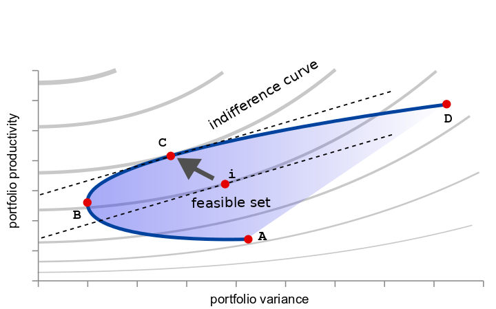
The problem objective is to choose the shares of different assets in the portfolio (here forest species, but the example is exactly the same considering other assets, for example financial investments) that maximise the portfolio expected returns while minimising its expected variance under the portfolio owner risk aversion risk. Here the "returns" are based on the timber production and the covariance between individual species of the portfolio is based on the observed volume growth covariances. The idea is that within the infinite possible allocations, the locus of those allocations for which is not possible to increase the portfolio profitability without increasing also its variance and the converse whose variance can not be lowered without at the same time lower its expected profitability are efficient in the Pareto meaning and form an "efficient frontier". Within this frontier the problem is to find the unique point that maximise the utility of the portfolio's owner given its risk aversion characteristic. Graphically the problem is depicted i nthe following picture:

The efficient frontier and the owner utility curves

Data originally from the Institut national de l'information géographique et forestière (IGN) of France. See the paper A. Dragicevic, A. Lobianco, A. Leblois (2016), ”Forest planning and productivity-risk trade-off through the Markowitz mean-variance model“, Forest Policy and Economics, Volume 64 for a thorough discussion of this model.

Declare the packages we are going to use:

julia> using JuMP, Ipopt, StatsPlots

Forest species names

julia> species   = ["Chêne pédonculé", "Chêne sessile", "Hêtre", "Pin sylvestre"]4-element Vector{String}:
 "Chêne pédonculé"
 "Chêne sessile"
 "Hêtre"
 "Pin sylvestre"
julia> nSpecies  = length(species)4

Average productiities by specie This is implemented in a dictionary: key->value

julia> y   = Dict( "Chêne pédonculé" => 1.83933333333333,
                   "Chêne sessile"   => 2.198,
                   "Hêtre"           => 3.286,
                   "Pin sylvestre"   => 3.3695)Dict{String, Float64} with 4 entries:
  "Hêtre"           => 3.286
  "Chêne pédonculé" => 1.83933
  "Chêne sessile"   => 2.198
  "Pin sylvestre"   => 3.3695

Covariance matrix between species

julia> σtable = [[0.037502535947712	0.016082745098039	0.027797176470588	-0.025589882352942]
                 [0.016082745098039	0.015177019607843	0.018791960784314	-0.102880470588234]
                 [0.027797176470588	0.018791960784314	0.031732078431373	-0.166391058823529]
                 [-0.025589882352942	-0.102880470588234	-0.166391058823529	2.02950454411765]]4×4 Matrix{Float64}:
  0.0375025   0.0160827   0.0277972  -0.0255899
  0.0160827   0.015177    0.018792   -0.10288
  0.0277972   0.018792    0.0317321  -0.166391
 -0.0255899  -0.10288    -0.166391    2.0295

We reshape the covariance matrix in a dictionary (sp1,sp2) -> value The function (ix,x) = enumerate(X) returns a tuple of index position and element for each element of an array

julia> σ = Dict((i,j) => σtable[i_ix,j_ix] for (i_ix,i) in enumerate(species), (j_ix,j) in enumerate(species))Dict{Tuple{String, String}, Float64} with 16 entries:
  ("Pin sylvestre", "Chêne pédonculé")   => -0.0255899
  ("Hêtre", "Chêne pédonculé")           => 0.0277972
  ("Chêne pédonculé", "Chêne sessile")   => 0.0160827
  ("Chêne pédonculé", "Pin sylvestre")   => -0.0255899
  ("Chêne pédonculé", "Hêtre")           => 0.0277972
  ("Hêtre", "Pin sylvestre")             => -0.166391
  ("Pin sylvestre", "Chêne sessile")     => -0.10288
  ("Chêne pédonculé", "Chêne pédonculé") => 0.0375025
  ("Hêtre", "Chêne sessile")             => 0.018792
  ("Chêne sessile", "Hêtre")             => 0.018792
  ("Hêtre", "Hêtre")                     => 0.0317321
  ("Chêne sessile", "Pin sylvestre")     => -0.10288
  ("Pin sylvestre", "Hêtre")             => -0.166391
  ("Pin sylvestre", "Pin sylvestre")     => 2.0295
  ("Chêne sessile", "Chêne sessile")     => 0.015177
  ("Chêne sessile", "Chêne pédonculé")   => 0.0160827

Showing the possible mean/variance of the portfolio by simulation

julia> nSamples = 10001000
julia> shares   = rand(nSamples,nSpecies);

Converting to probabilities:

julia> import BetaML.Utils:softmax
julia> [shares[i,:]  = softmax(shares[i,:], β=one.(shares[i,:]) .* 5) for i in 1:nSamples]1000-element Vector{Vector{Float64}}:
 [0.17335153349707058, 0.2028544675507532, 0.434853465506999, 0.1889405334451771]
 [0.4601396033380132, 0.0849324404589254, 0.23537950092368787, 0.21954845527937344]
 [0.09480772949506396, 0.06159560973824434, 0.7648357423116481, 0.07876091845504399]
 [0.5116176113263505, 0.19309546678940034, 0.2867535849204673, 0.008533336963781557]
 [0.6122479431894607, 0.2282432421083637, 0.06260752379342235, 0.09690129090875335]
 [0.05008657146368862, 0.7627679337377523, 0.17240550372262198, 0.014739991075937339]
 [0.2105918684267626, 0.08388276278270886, 0.37234222690347585, 0.3331831418870528]
 [0.07693605488874525, 0.1814900231552367, 0.5208361577817977, 0.2207377641742205]
 [0.5727338753842612, 0.03746180673429663, 0.36669006219356803, 0.023114255687873984]
 [0.0523981660364178, 0.6385708675052919, 0.2737816178191614, 0.035249348639129145]
 ⋮
 [0.06005044033498477, 0.21850759989252627, 0.2760058373164056, 0.4454361224560831]
 [0.05035647283628192, 0.03252865752680968, 0.466383545659842, 0.4507313239770662]
 [0.07918853957579651, 0.5757973750624649, 0.069428478913596, 0.27558560644814223]
 [0.08592761925553993, 0.8126387424868359, 0.060322985713022845, 0.041110652544601584]
 [0.09034681948863363, 0.3822532149770719, 0.029919722104154608, 0.4974802434301397]
 [0.20398814807426108, 0.01633929820820466, 0.12360307172602164, 0.6560694819915123]
 [0.15978026887646096, 0.28198295206216994, 0.04665986505228694, 0.5115769140090825]
 [0.5466085579201683, 0.1153800798635625, 0.29973186045636135, 0.03827950175990808]
 [0.0148204712124551, 0.020651551458972635, 0.3938682934030551, 0.5706596839255174]
julia> pScores = Array{Float64,2}(undef,0,2)0×2 Matrix{Float64}
julia> for i in 1:nSamples
           global pScores
           pVar    = sum(shares[i,j1] * shares[i,j2] * σ[species[j1],species[j2]] for j1 in 1:nSpecies, j2 in 1:nSpecies)
           pY      = sum(shares[i,j]*y[species[j]] for j in 1:nSpecies)
           pScores = vcat(pScores,[pVar pY])
       end
julia> scatter(pScores[:,1],pScores[:,2],colour=:blue)Plot{Plots.GRBackend() n=1}

Finding (one) optimal portfolio

Risk aversion coefficient

julia> α = 0.10.1

We declare an optimisation problem, we name it "m" and we let JuMP associate it with the most suitable solver within the one installed:

julia> port = Model(Ipopt.Optimizer)A JuMP Model
Feasibility problem with:
Variables: 0
Model mode: AUTOMATIC
CachingOptimizer state: EMPTY_OPTIMIZER
Solver name: Ipopt

We declare a set of variables, indicized by the species name:

julia> @variables port begin
           x[i in species] >= 0
       end(1-dimensional DenseAxisArray{JuMP.VariableRef,1,...} with index sets:
    Dimension 1, ["Chêne pédonculé", "Chêne sessile", "Hêtre", "Pin sylvestre"]
And data, a 4-element Vector{JuMP.VariableRef}:
 x[Chêne pédonculé]
 x[Chêne sessile]
 x[Hêtre]
 x[Pin sylvestre],)

We declare the constraint shat the sum of shares must be equal to 1

julia> @constraint(port, c_share, sum(x[i] for i in species) == 1)c_share : x[Chêne pédonculé] + x[Chêne sessile] + x[Hêtre] + x[Pin sylvestre] = 1
julia> @NLobjective port Min α *  sum(x[i] * x[j] * σ[i,j] for i in species for j in species) - sum(x[i] * y[i] for i in species)

Print the optimisation model in nice human-readable format:

julia> print(port)Min 0.1 * (x[Chêne pédonculé] * x[Chêne pédonculé] * 0.037502535947712 + x[Chêne pédonculé] * x[Chêne sessile] * 0.016082745098039 + x[Chêne pédonculé] * x[Hêtre] * 0.027797176470588 + x[Chêne pédonculé] * x[Pin sylvestre] * -0.025589882352942 + x[Chêne sessile] * x[Chêne pédonculé] * 0.016082745098039 + x[Chêne sessile] * x[Chêne sessile] * 0.015177019607843 + x[Chêne sessile] * x[Hêtre] * 0.018791960784314 + x[Chêne sessile] * x[Pin sylvestre] * -0.102880470588234 + x[Hêtre] * x[Chêne pédonculé] * 0.027797176470588 + x[Hêtre] * x[Chêne sessile] * 0.018791960784314 + x[Hêtre] * x[Hêtre] * 0.031732078431373 + x[Hêtre] * x[Pin sylvestre] * -0.166391058823529 + x[Pin sylvestre] * x[Chêne pédonculé] * -0.025589882352942 + x[Pin sylvestre] * x[Chêne sessile] * -0.102880470588234 + x[Pin sylvestre] * x[Hêtre] * -0.166391058823529 + x[Pin sylvestre] * x[Pin sylvestre] * 2.02950454411765) - (x[Chêne pédonculé] * 1.83933333333333 + x[Chêne sessile] * 2.198 + x[Hêtre] * 3.286 + x[Pin sylvestre] * 3.3695)
Subject to
 c_share : x[Chêne pédonculé] + x[Chêne sessile] + x[Hêtre] + x[Pin sylvestre] = 1
 x[Chêne pédonculé] ≥ 0
 x[Chêne sessile] ≥ 0
 x[Hêtre] ≥ 0
 x[Pin sylvestre] ≥ 0

Solve the model and return the solving status:

julia> optimize!(port)This is Ipopt version 3.14.13, running with linear solver MUMPS 5.6.1.

Number of nonzeros in equality constraint Jacobian...:        4
Number of nonzeros in inequality constraint Jacobian.:        0
Number of nonzeros in Lagrangian Hessian.............:       10

Total number of variables............................:        4
                     variables with only lower bounds:        4
                variables with lower and upper bounds:        0
                     variables with only upper bounds:        0
Total number of equality constraints.................:        1
Total number of inequality constraints...............:        0
        inequality constraints with only lower bounds:        0
   inequality constraints with lower and upper bounds:        0
        inequality constraints with only upper bounds:        0

iter    objective    inf_pr   inf_du lg(mu)  ||d||  lg(rg) alpha_du alpha_pr  ls
   0 -1.0691173e-01 9.60e-01 8.33e-01  -1.0 0.00e+00    -  0.00e+00 0.00e+00   0
   1 -2.6796169e+00 0.00e+00 2.26e+01  -1.7 2.46e-01    -  4.19e-02 1.00e+00f  1
   2 -3.2598524e+00 0.00e+00 2.13e+01  -1.7 6.87e+00    -  4.95e-02 5.88e-02f  1
   3 -3.2590630e+00 1.11e-16 1.93e+01  -1.7 1.61e-01    -  1.00e+00 9.81e-02f  2
   4 -3.2586433e+00 0.00e+00 2.00e-07  -1.7 1.45e-02    -  1.00e+00 1.00e+00f  1
   5 -3.2971652e+00 0.00e+00 4.96e-03  -3.8 7.04e-02    -  9.08e-01 1.00e+00f  1
   6 -3.2983547e+00 0.00e+00 1.50e-09  -3.8 2.19e-02    -  1.00e+00 1.00e+00f  1
   7 -3.2986538e+00 0.00e+00 1.84e-11  -5.7 2.93e-03    -  1.00e+00 1.00e+00f  1
   8 -3.2986576e+00 0.00e+00 2.55e-14  -8.6 4.72e-05    -  1.00e+00 1.00e+00f  1

Number of Iterations....: 8

                                   (scaled)                 (unscaled)
Objective...............:  -3.2986575928648394e+00   -3.2986575928648394e+00
Dual infeasibility......:   2.5521078983849546e-14    2.5521078983849546e-14
Constraint violation....:   0.0000000000000000e+00    0.0000000000000000e+00
Variable bound violation:   8.2731345336654260e-09    8.2731345336654260e-09
Complementarity.........:   3.5155177510884357e-09    3.5155177510884357e-09
Overall NLP error.......:   3.5155177510884357e-09    3.5155177510884357e-09


Number of objective function evaluations             = 11
Number of objective gradient evaluations             = 9
Number of equality constraint evaluations            = 11
Number of inequality constraint evaluations          = 0
Number of equality constraint Jacobian evaluations   = 1
Number of inequality constraint Jacobian evaluations = 0
Number of Lagrangian Hessian evaluations             = 8
Total seconds in IPOPT                               = 1.397

EXIT: Optimal Solution Found.
julia> status = termination_status(port)LOCALLY_SOLVED::TerminationStatusCode = 4

Return the objective:

julia> println("Objective value: ", objective_value(port))Objective value: -3.2986575928648394

Return the value of the decision variable:

julia> optShares = value.(x)1-dimensional DenseAxisArray{Float64,1,...} with index sets:
    Dimension 1, ["Chêne pédonculé", "Chêne sessile", "Hêtre", "Pin sylvestre"]
And data, a 4-element Vector{Float64}:
 -8.273134533665426e-9
 -7.695921190269722e-9
  0.7428494846386048
  0.25715053133045096
julia> [println("$sp = $(optShares[sp])") for sp in species];Chêne pédonculé = -8.273134533665426e-9
Chêne sessile = -7.695921190269722e-9
Hêtre = 0.7428494846386048
Pin sylvestre = 0.25715053133045096
julia> pOptVar = sum(optShares[species[j1]] * optShares[species[j2]] * σ[species[j1],species[j2]] for j1 in 1:nSpecies, j2 in 1:nSpecies)0.0881449684288383
julia> pOptY   = sum(optShares[species[j]]*y[species[j]] for j in 1:nSpecies)3.307472089707723
julia> function computeOptimalPortfolio(species,y,σ,α)
           port = Model(Ipopt.Optimizer)
           set_optimizer_attribute(port, "print_level", 0)
           @variables port begin
               x[i in species] >= 0
           end
           @constraint(port, c_share, sum(x[i] for i in species) == 1)
           @NLobjective port Min α *  sum(x[i] * x[j] * σ[i,j] for i in species for j in species) - sum(x[i] * y[i] for i in species)
           optimize!(port)
           status = termination_status(port)
           optShares = value.(x)
           pOptVar = sum(optShares[species[j1]] * optShares[species[j2]] * σ[species[j1],species[j2]] for j1 in 1:nSpecies, j2 in 1:nSpecies)
           pOptY   = sum(optShares[species[j]]*y[species[j]] for j in 1:nSpecies)
           return (pOptVar,pOptY)
       endcomputeOptimalPortfolio (generic function with 1 method)
julia> αs = [1000,100,10,1,0.1,0.05,0.02,0.01]8-element Vector{Float64}:
 1000.0
  100.0
   10.0
    1.0
    0.1
    0.05
    0.02
    0.01
julia> pOptScores = Array{Float64,2}(undef,0,2)0×2 Matrix{Float64}
julia> for α in αs
           global pOptScores
           pVar,pY =computeOptimalPortfolio(species,y,σ,α)
           pOptScores = vcat(pOptScores,[pVar pY])
       end
julia> scatter!(pOptScores[:,1],pOptScores[:,2],colour=:red)Plot{Plots.GRBackend() n=2}

julia> αs = [82.45,50,30,20,15,12,10,9,8,7,6,5]12-element Vector{Float64}:
 82.45
 50.0
 30.0
 20.0
 15.0
 12.0
 10.0
  9.0
  8.0
  7.0
  6.0
  5.0
julia> pOptScores = Array{Float64,2}(undef,0,2)0×2 Matrix{Float64}
julia> for α in αs
           global pOptScores
           pVar,pY =computeOptimalPortfolio(species,y,σ,α)
           pOptScores = vcat(pOptScores,[pVar pY])
       end
julia> scatter(pOptScores[:,1],pOptScores[:,2],colour=:red)Plot{Plots.GRBackend() n=1}

View this file on Github.

This page was generated using Literate.jl.