A classification task when labels are known - determining the country of origin of cars given the cars' characteristics
In this exercise we are provided with several technical characteristics (mpg, horsepower,weight, model year...) for several car models, together with the country of origin of such models, and we would like to create a machine learning model such that the country of origin can be accurately predicted given the technical characteristics. As the information to predict is a multi-class one, this is a [classification](https://en.wikipedia.org/wiki/Statisticalclassification) task. It is a challenging exercise due to the simultaneous presence of three factors: (1) presence of missing data; (2) unbalanced data - 254 out of 406 cars are US made; (3) small dataset.
Data origin:
- dataset description: https://archive.ics.uci.edu/ml/datasets/auto+mpg
- data source we use here: https://archive.ics.uci.edu/ml/machine-learning-databases/auto-mpg/auto-mpg.data
Field description:
- mpg: continuous
- cylinders: multi-valued discrete
- displacement: continuous
- horsepower: continuous
- weight: continuous
- acceleration: continuous
- model year: multi-valued discrete
- origin: multi-valued discrete
- car name: string (unique for each instance)
The car name is not used in this tutorial, so that the country is inferred only from technical data. As this field also includes the car maker, and there are several car models from the same car maker, a more sophisticated machine learning model could exploit this information e.g. using a bag of words encoding.
Library loading and initialisation
Activating the local environment specific to BetaML documentation
using Pkg
Pkg.activate(joinpath(@__DIR__,"..","..",".."))
Activating project at `~/work/BetaML.jl/BetaML.jl/docs`We load a bunch of packages that we'll use during this tutorial.
using Random, HTTP, Plots, CSV, DataFrames, BenchmarkTools, StableRNGs, BetaML
import DecisionTree, Flux
import Pipe: @pipe
Machine Learning workflows include stochastic components in several steps: in the data sampling, in the model initialisation and often in the models' own algorithms (and sometimes also in the prediction step). BetaML provides a random number generator (RNG) in order to simplify reproducibility ( FIXEDRNG. This is nothing other than an instance of StableRNG(123) defined in the BetaML.Utils sub-module, but you can of course choose your own "fixed" RNG). See the Dealing with stochasticity section in the Getting started tutorial for details.
Here we are explicit and we use our own fixed RNG:
seed = 123 # The table at the end of this tutorial has been obtained with seeds 123, 1000 and 10000
AFIXEDRNG = StableRNG(seed)StableRNGs.LehmerRNG(state=0x000000000000000000000000000000f7)Data loading and preparation
To load the data from the internet our workflow is (1) Retrieve the data –> (2) Clean it –> (3) Load it –> (4) Output it as a DataFrame.
For step (1) we use HTTP.get(), for step (2) we use replace!, for steps (3) and (4) we use the CSV package, and we use the "pipe" |> operator to chain these operations, so that no file is ever saved on disk:
urlDataOriginal = "https://archive.ics.uci.edu/ml/machine-learning-databases/auto-mpg/auto-mpg.data-original"
data = @pipe HTTP.get(urlDataOriginal).body                                                |>
             replace!(_, UInt8('\t') => UInt8(' '))                                        |> # the original dataset has mixed field delimiters !
             CSV.File(_, delim=' ', missingstring="NA", ignorerepeated=true, header=false) |>
             DataFrame;
This results in a table where the rows are the observations (the various car models) and the columns the fields. All BetaML models expect this layout.
As the dataset is ordered, we randomly shuffle the data.
idx = randperm(copy(AFIXEDRNG),size(data,1))
data[idx, :]
describe(data)| Row | variable | mean | min | median | max | nmissing | eltype |
|---|---|---|---|---|---|---|---|
| Symbol | Union… | Any | Union… | Any | Int64 | Type | |
| 1 | Column1 | 23.5146 | 9.0 | 23.0 | 46.6 | 8 | Union{Missing, Float64} |
| 2 | Column2 | 5.47537 | 3.0 | 4.0 | 8.0 | 0 | Float64 |
| 3 | Column3 | 194.78 | 68.0 | 151.0 | 455.0 | 0 | Float64 |
| 4 | Column4 | 105.082 | 46.0 | 95.0 | 230.0 | 6 | Union{Missing, Float64} |
| 5 | Column5 | 2979.41 | 1613.0 | 2822.5 | 5140.0 | 0 | Float64 |
| 6 | Column6 | 15.5197 | 8.0 | 15.5 | 24.8 | 0 | Float64 |
| 7 | Column7 | 75.9212 | 70.0 | 76.0 | 82.0 | 0 | Float64 |
| 8 | Column8 | 1.56897 | 1.0 | 1.0 | 3.0 | 0 | Float64 |
| 9 | Column9 | amc ambassador brougham | vw rabbit custom | 0 | String |
Columns 1 to 7 contain characteristics of the car, while column 8 encodes the country of origin ("1" -> US, "2" -> EU, "3" -> Japan). That's the variable we want to be able to predict.
Column 9 contains the car name, but we are not going to use this information in this tutorial. Note also that some fields have missing data.
Our first step is hence to divide the dataset into features (the x) and the labels (the y) we want to predict. The x is then a Julia standard Matrix of 406 rows by 7 columns and the y is a vector of the 406 observations:
x     = Matrix{Union{Missing,Float64}}(data[:,1:7]);
y     = Vector{Int64}(data[:,8]);
x     = fit!(Scaler(),x)
406×7 Matrix{Union{Missing, Float64}}:
-0.706439 1.47635 1.07088 0.643526 0.620107 -1.25708 -1.58146
-1.09075 1.47635 1.48121 1.54744 0.843522 -1.43566 -1.58146
-0.706439 1.47635 1.17584 1.16005 0.539725 -1.61424 -1.58146
-0.962647 1.47635 1.04225 1.16005 0.536179 -1.25708 -1.58146
-0.834543 1.47635 1.02316 0.901788 0.555092 -1.79281 -1.58146
-1.09075 1.47635 2.23507 2.39971 1.60951 -1.97139 -1.58146
-1.21885 1.47635 2.47364 2.96789 1.62488 -2.32855 -1.58146
-1.21885 1.47635 2.34004 2.83876 1.57523 -2.50712 -1.58146
-1.21885 1.47635 2.48318 3.09702 1.70881 -1.97139 -1.58146
-1.09075 1.47635 1.86291 2.1931 1.02911 -2.50712 -1.58146
⋮ ⋮
-0.194023 0.306793 0.35518 0.178653 -0.17071 -0.292762 1.62356
1.08702 -0.862764 -0.484569 -0.234567 -0.371665 -0.578486 1.62356
1.59943 -0.862764 -0.570453 -0.544482 -0.720381 -0.899925 1.62356
0.446497 -0.862764 -0.417771 -0.389524 -0.0347697 0.635842 1.62356
0.446497 -0.862764 -0.52274 -0.492829 -0.223904 0.028678 1.62356
2.62426 -0.862764 -0.933072 -1.37092 -1.00408 3.24307 1.62356
1.08702 -0.862764 -0.570453 -0.544482 -0.809037 -1.39994 1.62356
0.574601 -0.862764 -0.713592 -0.673613 -0.418948 1.10014 1.62356
0.958913 -0.862764 -0.723135 -0.596135 -0.30665 1.38587 1.62356Some algorithms that we will use today don't accept missing data, so we need to impute them. BetaML provides several imputation models in the Imputation module. Note that many of these imputation models can be used for Collaborative Filtering / Recommendation Systems. Models such as GaussianMixtureImputer have the advantage over traditional algorithms such as k-nearest neighbors (KNN) that GMM can "detect" the hidden structure of the observed data, where some observations can be similar to a certain pool of other observations for a certain characteristic, but similar to another pool of observations for other characteristics. Here we use RandomForestImputer. While the model allows for reproducible multiple imputations (with the parameter multiple_imputation=an_integer) and multiple passages through the various columns (fields) containing missing data (with the option recursive_passages=an_integer), we use here just a single imputation and a single passage. As all BetaML models, RandomForestImputer follows the pattern m=ModelConstruction(pars); fit!(m,x,[y]); est = predict(m,x) where est can be an estimation of some labels or be some characteristics of x itself (the imputed version, as in this case, a reprojected version as in PCAEncoder), depending on whether the model is supervised or not. See the API user documentation for more details. For imputers, the output of predict is the matrix with the imputed values replacing the missing ones, and we write here the model in a single line using a convenience feature that when the default cache parameter is used in the model constructor the fit! function itself returns the prediction over the trained data:
x = fit!(RandomForestImputer(rng=copy(AFIXEDRNG)),x) # Same as `m = RandomForestImputer(rng=copy(AFIXEDRNG)); fit!(m,x); x= predict(m,x)`406×7 Matrix{Float64}:
-0.706439 1.47635 1.07088 0.643526 0.620107 -1.25708 -1.58146
-1.09075 1.47635 1.48121 1.54744 0.843522 -1.43566 -1.58146
-0.706439 1.47635 1.17584 1.16005 0.539725 -1.61424 -1.58146
-0.962647 1.47635 1.04225 1.16005 0.536179 -1.25708 -1.58146
-0.834543 1.47635 1.02316 0.901788 0.555092 -1.79281 -1.58146
-1.09075 1.47635 2.23507 2.39971 1.60951 -1.97139 -1.58146
-1.21885 1.47635 2.47364 2.96789 1.62488 -2.32855 -1.58146
-1.21885 1.47635 2.34004 2.83876 1.57523 -2.50712 -1.58146
-1.21885 1.47635 2.48318 3.09702 1.70881 -1.97139 -1.58146
-1.09075 1.47635 1.86291 2.1931 1.02911 -2.50712 -1.58146
⋮ ⋮
-0.194023 0.306793 0.35518 0.178653 -0.17071 -0.292762 1.62356
1.08702 -0.862764 -0.484569 -0.234567 -0.371665 -0.578486 1.62356
1.59943 -0.862764 -0.570453 -0.544482 -0.720381 -0.899925 1.62356
0.446497 -0.862764 -0.417771 -0.389524 -0.0347697 0.635842 1.62356
0.446497 -0.862764 -0.52274 -0.492829 -0.223904 0.028678 1.62356
2.62426 -0.862764 -0.933072 -1.37092 -1.00408 3.24307 1.62356
1.08702 -0.862764 -0.570453 -0.544482 -0.809037 -1.39994 1.62356
0.574601 -0.862764 -0.713592 -0.673613 -0.418948 1.10014 1.62356
0.958913 -0.862764 -0.723135 -0.596135 -0.30665 1.38587 1.62356Further, some models don't work with categorical data as well, so we need to represent our y as a matrix with a separate column for each possible categorical value (the so-called "one-hot" representation). For example, within a three-class field, the individual value 2 (or "Europe" for that matter) would be represented as the vector [0 1 0], while 3 (or "Japan") would become the vector [0 0 1]. To encode as one-hot we use the OneHotEncoder in BetaML.Utils, using the same shortcut as for the imputer we used earlier:
y_oh = fit!(OneHotEncoder(),y)406×3 Matrix{Bool}:
1 0 0
1 0 0
1 0 0
1 0 0
1 0 0
1 0 0
1 0 0
1 0 0
1 0 0
1 0 0
⋮
1 0 0
0 0 1
1 0 0
1 0 0
1 0 0
0 1 0
1 0 0
1 0 0
1 0 0In supervised machine learning it is good practice to partition the available data into training, validation, and test subsets, where the first one is used to train the ML algorithm, the second one to train any "hyper-parameters" of the algorithm and the test subset is finally used to evaluate the quality of the algorithm. Here, for brevity, we use only the train and the test subsets, implicitly assuming we already know the best hyper-parameters. Please refer to the regression tutorial for examples of the auto-tune feature of BetaML models to "automatically" train the hyper-parameters (hint: in most cases just add the parameter autotune=true in the model constructor), or the clustering tutorial for an example of using the cross_validation function to do it manually.
We then use the partition function in BetaML.Utils, where we can specify the different data to partition (each matrix or vector to partition must have the same number of observations) and the shares of observations that we want in each subset. Here we keep 80% of observations for training (xtrain, and ytrain) and we use 20% of them for testing (xtest, and ytest):
((xtrain,xtest),(ytrain,ytest),(ytrain_oh,ytest_oh)) = partition([x,y,y_oh],[0.8,1-0.8],rng=copy(AFIXEDRNG));We finally set up a dataframe to store the accuracies of the various models we'll use.
results = DataFrame(model=String[],train_acc=Float64[],test_acc=Float64[])| Row | model | train_acc | test_acc |
|---|---|---|---|
| String | Float64 | Float64 |
Random Forests
We are now ready to use our first model, the RandomForestEstimator. Random Forests build a "forest" of decision tree models and then average their predictions in order to make an overall prediction, whether a regression or a classification.
While here the missing data has been imputed and the dataset is comprised of only numerical values, one attractive feature of BetaML RandomForestEstimator is that it can work directly with missing and categorical data without any prior processing required.
However as the labels are encoded using integers, we also need to specify the parameter force_classification=true, otherwise the model would perform a regression job instead.
rfm = RandomForestEstimator(force_classification=true, rng=copy(AFIXEDRNG))RandomForestEstimator - A 30 trees Random Forest model (unfitted)Unlike the RandomForestImputer and OneHotEncoder models used earlier, to train a RandomForestEstimator model we need to provide it with both the training feature matrix and the associated "true" training labels. We use the same shortcut to get the training predictions directly from the fit! function. In this case the predictions correspond to the labels:
ŷtrain = fit!(rfm,xtrain,ytrain)325-element Vector{Dict{Int64, Float64}}:
Dict(3 => 0.9333333333333332, 2 => 0.03333333333333333, 1 => 0.03333333333333333)
Dict(1 => 0.9999999999999999)
Dict(3 => 0.1, 2 => 0.8999999999999999)
Dict(3 => 0.1, 2 => 0.016666666666666666, 1 => 0.8833333333333332)
Dict(3 => 0.13333333333333333, 2 => 0.6833333333333332, 1 => 0.18333333333333332)
Dict(1 => 0.9999999999999999)
Dict(3 => 0.8499999999999999, 2 => 0.11666666666666667, 1 => 0.03333333333333333)
Dict(1 => 0.9999999999999999)
Dict(3 => 0.03333333333333333, 1 => 0.9666666666666666)
Dict(3 => 0.05, 2 => 0.4833333333333333, 1 => 0.4666666666666666)
⋮
Dict(1 => 0.9999999999999999)
Dict(3 => 0.8333333333333333, 2 => 0.16666666666666666)
Dict(1 => 0.9999999999999999)
Dict(1 => 0.9999999999999999)
Dict(1 => 0.9999999999999999)
Dict(3 => 0.08333333333333334, 2 => 0.8166666666666665, 1 => 0.1)
Dict(1 => 0.9999999999999999)
Dict(3 => 0.9499999999999998, 2 => 0.05)
Dict(3 => 0.8666666666666666, 2 => 0.1, 1 => 0.03333333333333333)You can notice that for each record the result is reported in terms of a dictionary with the possible categories and their associated probabilities.
Only categories with non-zero probabilities are reported for each record, and being a dictionary, the order of the categories is undefined
For example ŷtrain[1] is a Dict(2 => 0.0333333, 3 => 0.933333, 1 => 0.0333333), indicating an overwhelming probability that that car model originates from Japan. To retrieve the predictions with the highest probabilities use mode(ŷ):
ŷtrain_top = mode(ŷtrain,rng=copy(AFIXEDRNG))325-element Vector{Int64}:
3
1
2
1
2
1
3
1
1
2
⋮
1
3
1
1
1
2
1
3
3Why does mode (optionally) take an RNG? I leave the answer to you :-)
To obtain the predicted labels for the test set we simply run the predict function over the features of the test set:
ŷtest = predict(rfm,xtest)81-element Vector{Dict{Int64, Float64}}:
Dict(3 => 0.08333333333333333, 2 => 0.5499999999999999, 1 => 0.36666666666666664)
Dict(3 => 0.1, 2 => 0.7166666666666667, 1 => 0.18333333333333332)
Dict(3 => 0.03333333333333333, 2 => 0.6, 1 => 0.36666666666666664)
Dict(1 => 0.9999999999999999)
Dict(3 => 0.15, 2 => 0.16666666666666666, 1 => 0.6833333333333332)
Dict(1 => 0.9999999999999999)
Dict(3 => 0.7, 2 => 0.26666666666666666, 1 => 0.03333333333333333)
Dict(3 => 0.3, 2 => 0.5833333333333333, 1 => 0.11666666666666667)
Dict(2 => 0.05, 1 => 0.9499999999999998)
Dict(1 => 0.9999999999999999)
⋮
Dict(3 => 0.06666666666666667, 2 => 0.24999999999999997, 1 => 0.6833333333333332)
Dict(1 => 0.9999999999999999)
Dict(3 => 0.6333333333333333, 2 => 0.3, 1 => 0.06666666666666667)
Dict(1 => 0.9999999999999999)
Dict(1 => 0.9999999999999999)
Dict(3 => 0.3333333333333333, 2 => 0.06666666666666667, 1 => 0.6)
Dict(3 => 0.9999999999999999)
Dict(3 => 0.4333333333333333, 2 => 0.19999999999999998, 1 => 0.36666666666666664)
Dict(1 => 0.9999999999999999)Finally we can measure the accuracy of our predictions with the accuracy function. We don't need to explicitly use mode, as accuracy does it itself when it is passed predictions expressed as a dictionary:
trainAccuracy,testAccuracy = accuracy.([ytrain,ytest],[ŷtrain,ŷtest],rng=copy(AFIXEDRNG))2-element Vector{Float64}:
0.9969230769230769
0.7530864197530864We are now ready to store our first model accuracies in the results dataframe:
push!(results,["RF",trainAccuracy,testAccuracy]);The predictions are quite good, for the training set the algorithm predicted almost all cars' origins correctly, while for the testing set (i.e. those records that have not been used to train the algorithm), the correct prediction level is still quite high, at around 80% (depending on the random seed)
While accuracy can sometimes suffice, we may often want to better understand which categories our model has trouble predicting correctly. We can investigate the output of a multi-class classifier more in depth with a ConfusionMatrix where the true values (y) are given in rows and the predicted ones (ŷ) in columns, together with some per-class metrics like the precision (true class i over predicted in class i), the recall (predicted class i over the true class i) and others.
We first build the ConfusionMatrix model, we train it with ŷ and y and then we print it (we do it here for the test subset):
cfm = ConfusionMatrix(categories_names=Dict(1=>"US",2=>"EU",3=>"Japan"),rng=copy(AFIXEDRNG))
fit!(cfm,ytest,ŷtest) # the output is by default the confusion matrix in relative terms
print(cfm)
A ConfusionMatrix BetaMLModel (fitted)
-----------------------------------------------------------------
*** CONFUSION MATRIX ***
Scores actual (rows) vs predicted (columns):
4×4 Matrix{Any}:
"Labels" "EU" "US" "Japan"
"EU" 10 4 2
"US" 2 45 2
"Japan" 3 7 6
Normalised scores actual (rows) vs predicted (columns):
4×4 Matrix{Any}:
"Labels" "EU" "US" "Japan"
"EU" 0.625 0.25 0.125
"US" 0.0408163 0.918367 0.0408163
"Japan" 0.1875 0.4375 0.375
*** CONFUSION REPORT ***
- Accuracy: 0.7530864197530864
- Misclassification rate: 0.24691358024691357
- Number of classes: 3
N Class precision recall specificity f1score actual_count predicted_count
TPR TNR support
1 EU 0.667 0.625 0.923 0.645 16 15
2 US 0.804 0.918 0.656 0.857 49 56
3 Japan 0.600 0.375 0.938 0.462 16 10
- Simple avg. 0.690 0.639 0.839 0.655
- Weighted avg. 0.736 0.753 0.765 0.737
-----------------------------------------------------------------
Output of `info(cm)`:
- normalised_scores: [0.625 0.25 0.125; 0.04081632653061224 0.9183673469387755 0.04081632653061224; 0.1875 0.4375 0.375]
- n_categories: 3
- fp: [5, 11, 4]
- tn: [60, 21, 61]
- predicted_count: [15, 56, 10]
- scores: [10 4 2; 2 45 2; 3 7 6]
- mean_f1score: (0.6546142030012998, 0.7371258769108231)
- fitted_records: 81
- recall: [0.625, 0.9183673469387755, 0.375]
- actual_count: [16, 49, 16]
- fn: [6, 4, 10]
- f1score: [0.6451612903225806, 0.8571428571428571, 0.46153846153846156]
- accuracy: 0.7530864197530864
- mean_recall: (0.6394557823129251, 0.7530864197530864)
- mean_specificity: (0.8392628205128205, 0.7647020417853753)
- misclassification: 0.24691358024691357
- precision: [0.6666666666666666, 0.8035714285714286, 0.6]
- categories: ["EU", "US", "Japan"]
- specificity: [0.9230769230769231, 0.65625, 0.9384615384615385]
- tp: [10, 45, 6]
- mean_precision: (0.6900793650793652, 0.7363168724279835)From the report we can see that Japanese cars have more trouble being correctly classified, and in particular many Japanese cars are classified as US ones. This is likely a result of the class imbalance of the data set, and could be solved by balancing the dataset with various sampling techniques before training the model.
If you prefer a more graphical approach, we can also plot the confusion matrix. In order to do so, we pick up information from the info(cfm) function. Indeed most BetaML models can be queried with info(model) to retrieve additional information, in terms of a dictionary, that is not necessary for the prediction, but could still be relevant. Other functions that you can use with BetaML models are parameters(m) and hyperparameters(m).
res = info(cfm)
heatmap(string.(res["categories"]),string.(res["categories"]),res["normalised_scores"],seriescolor=cgrad([:white,:blue]),xlabel="Predicted",ylabel="Actual", title="Confusion Matrix (normalised scores)")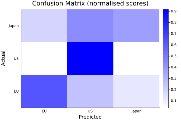
Comparison with DecisionTree.jl
We now compare BetaML [RandomForestEstimator] with the random forest estimator of the package DecisionTrees.jl, whose random forests are similar in usage: we first "build" (train) the forest and we then make predictions out of the trained model.
# We train the model...
model = DecisionTree.build_forest(ytrain, xtrain,rng=seed)
# ..and we generate predictions and measure their error
(ŷtrain,ŷtest) = DecisionTree.apply_forest.([model],[xtrain,xtest]);
(trainAccuracy,testAccuracy) = accuracy.([ytrain,ytest],[ŷtrain,ŷtest])
push!(results,["RF (DecisionTrees.jl)",trainAccuracy,testAccuracy]);
DecisionTree.jl random forests reach an accuracy similar to, but generally slightly lower than, that of BetaML random forests (see the summary table at the end of this tutorial). Where DecisionTrees.jl excels, however, is in efficiency: they are extremely fast and memory thrifty, even if we should consider also the resources needed to impute the missing values, as they don't work with missing data.
Also, one of the reasons DecisionTrees are so efficient is that internally the data is sorted to avoid repeated comparisons, but in this way they work only with features that are sortable, while BetaML random forests accept virtually any kind of input without the need to process it.
Neural network
Neural networks (NN) can be very powerful, but have two "inconveniences" compared with random forests: first, they are a bit "picky". We need to do a bit of work to provide data in a specific format. Note that this is not feature engineering. One of the advantages of neural networks is that for the most part this is not needed. However we still need to "clean" the data. One issue is that NN don't like missing data. So we need to provide them with the feature matrix "clean" of missing data. Secondly, they work only with numerical data. So we need to use the one-hot encoding we saw earlier. Further, they work best if the features are scaled such that each feature has mean zero and standard deviation 1. This is why we scaled the data back at the beginning of this tutorial.
We first measure the dimensions of our data in input (i.e. the columns of the feature matrix) and the dimensions of our output, i.e. the number of categories or columns in our one-hot encoded y.
D               = size(xtrain,2)
classes         = unique(y)
nCl = length(classes)3The second "inconvenience" of NN is that, while not requiring feature engineering, they still need a bit of practice on the way the structure of the network is built. It's not as simple as fit!(Model(),x,y) (although BetaML provides a "default" neural network structure that can be used, it often isn't adapted to the specific task). We need instead to specify how we want our layers, chain the layers together and then decide an overall loss function. Only when we have done these steps, we have the model ready for training. Here we define 2 DenseLayer where, for each of them, we specify the number of neurons in input (the first layer being equal to the dimensions of the data), the output layer (for a classification task, the last layer output size being equal to the number of classes) and an activation function for each layer (by default the identity function).
ls   = 50 # number of neurons in the inner layer
l1   = DenseLayer(D,ls,f=relu,rng=copy(AFIXEDRNG))
l2   = DenseLayer(ls,nCl,f=relu,rng=copy(AFIXEDRNG))
DenseLayer{typeof(relu), typeof(drelu), Float64, Matrix{Float64}, Vector{Float64}}([-0.2146463925907584 -0.3077087587320811 … -0.28256208289474877 0.21510681158042189; -0.08916953797649538 -0.041727530915651345 … -0.30444064706465346 -0.22349634154766507; 0.11376391271810127 -0.011244515923068743 … 0.12916068649773038 -0.2518581440082599], [0.2918467648814228, -0.004167534280141383, 0.29060333096888613], BetaML.Utils.relu, BetaML.Utils.drelu)For a classification task, the last layer is a VectorFunctionLayer that has no learnable parameters but whose activation function is applied to the ensemble of the neurons, rather than individually on each neuron. In particular, for classification we pass the softmax function whose output has the same size as the input (i.e. the number of classes to predict), but we can use the VectorFunctionLayer with any function. For example, for a "pooling" layer we could use the pool1d function (although for pooling with maximum or mean the PoolingLayer is more efficient)
l3 = VectorFunctionLayer(nCl,f=softmax) ## Add a (parameterless) layer whose activation function (softmax in this case) is applied to all its nodes at onceVectorFunctionLayer{0, typeof(softmax), typeof(dsoftmax), Nothing, Float64, Array{Float64, 0}}(fill(NaN), 3, 3, BetaML.Utils.softmax, BetaML.Utils.dsoftmax, nothing, false)Finally we chain the layers and assign a loss function and the number of epochs we want to train the model to the constructor of NeuralNetworkEstimator:
nn = NeuralNetworkEstimator(layers=[l1,l2,l3],loss=crossentropy,rng=copy(AFIXEDRNG),epochs=500)NeuralNetworkEstimator - A Feed-forward neural network (unfitted)Aside from the layer structure and size and the number of epochs, other hyper-parameters you may want to try are the batch_size and the optimisation algorithm to employ (opt_alg).
Now we can train our network:
ŷtrain = fit!(nn, xtrain, ytrain_oh)325×3 Matrix{Float64}:
0.0676677 0.0275345 0.904798
0.999972 1.81974e-5 9.92836e-6
0.00779478 0.954113 0.0380927
0.58527 0.207365 0.207365
0.00437752 0.903605 0.0920178
1.0 6.09325e-9 9.40566e-11
0.251525 0.106944 0.641531
1.0 1.56965e-15 2.67547e-15
0.999994 4.86833e-6 9.11529e-7
0.623723 0.322994 0.0532836
⋮
1.0 4.02462e-13 1.65826e-13
0.179315 0.179315 0.641371
1.0 8.71747e-8 8.71747e-8
0.991984 0.00400818 0.00400818
1.0 3.65242e-12 3.61968e-12
0.488085 0.491104 0.0208112
1.0 5.90875e-14 9.12098e-16
0.0887457 0.0887457 0.822509
0.0356859 0.00917201 0.955142Predictions are in the form of a nrecords_ by nclasses_ matrix of the probabilities of each record being in that class. To retrieve the classes with the highest probabilities we can use again the mode function:
ŷtrain_top = mode(ŷtrain)325-element Vector{Int64}:
3
1
2
1
2
1
3
1
1
1
⋮
1
3
1
1
1
2
1
3
3Once trained, we can predict the test labels. As the training was based on the scaled feature matrix, so must the predictions be
ŷtest = predict(nn,xtest)81×3 Matrix{Float64}:
0.000624716 0.99936 1.54372e-5
6.69106e-5 0.999931 1.60829e-6
0.118704 0.0481194 0.833177
1.0 1.0696e-11 1.0696e-11
0.134997 0.0333475 0.831655
1.0 2.61403e-9 2.61403e-9
0.0628621 0.0388272 0.898311
0.319803 0.319803 0.360394
0.864846 0.0675768 0.0675768
1.0 6.14318e-9 2.08419e-11
⋮
0.909121 0.0454397 0.0454397
1.0 6.73847e-14 4.67989e-14
0.025709 0.0446431 0.929648
1.0 1.35308e-9 1.04677e-11
1.0 2.62551e-11 5.72552e-11
0.420121 0.0408367 0.539042
0.0677272 0.0574378 0.874835
0.000173391 0.999636 0.000190466
1.0 9.2729e-9 9.2729e-9And finally we can measure the accuracies and store the accuracies in the result dataframe:
trainAccuracy, testAccuracy   = accuracy.([ytrain,ytest],[ŷtrain,ŷtest],rng=copy(AFIXEDRNG))
push!(results,["NN",trainAccuracy,testAccuracy]);
cfm = ConfusionMatrix(categories_names=Dict(1=>"US",2=>"EU",3=>"Japan"),rng=copy(AFIXEDRNG))
fit!(cfm,ytest,ŷtest)
print(cfm)
res = info(cfm)
heatmap(string.(res["categories"]),string.(res["categories"]),res["normalised_scores"],seriescolor=cgrad([:white,:blue]),xlabel="Predicted",ylabel="Actual", title="Confusion Matrix (normalised scores)")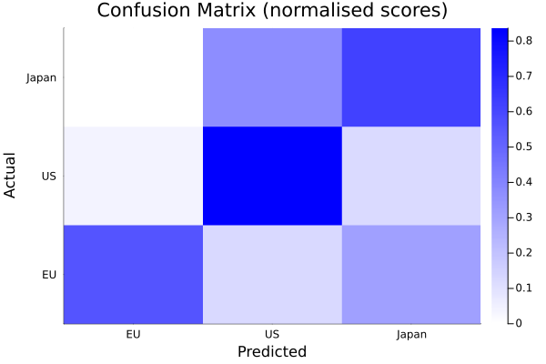
While accuracies are a bit lower, the distribution of misclassification is similar, with many Japanese cars misclassified as US ones (here we have also some EU cars misclassified as Japanese ones).
Comparisons with Flux
As we did for Random Forests, we compare BetaML neural networks with the leading package for deep learning in Julia, Flux.jl.
In Flux the input must be in the form (fields, observations), so we transpose our original matrices. We also convert the features to Float32, the type of the Flux model parameters:
xtrainT, ytrain_ohT = Float32.(permutedims(xtrain)), permutedims(ytrain_oh)
xtestT, ytest_ohT   = Float32.(permutedims(xtest)), permutedims(ytest_oh)
(Float32[-0.93702585 0.830809 … 1.6506745 -0.57833475; 0.30679256 -0.86276406 … -0.27798575 0.30679256; … ; 0.10010898 2.2430394 … 1.5644448 -0.007037538; 0.55522233 1.0893935 … 1.0893935 -1.314377], Bool[0 0 … 0 1; 1 1 … 1 0; 0 0 … 0 0])We define the Flux neural network model in a similar way to BetaML and load it with data, we train it, predict and measure the accuracies on the training and the test sets. We use the "explicit" Flux API: the loss function takes the model as its first argument, and the state of the optimisation algorithm is set up once, before the training loop, with Flux.setup:
We fix the random seed for Flux, although you may still get different results depending on the number of threads used... this is a problem we solve in BetaML by creating a master seed and then reseeding with it each parallel computation.
Random.seed!(seed)

Flux_nn    = Flux.Chain(Flux.Dense(D,ls,Flux.relu),Flux.Dense(ls,nCl,Flux.relu))
fluxloss(m, x, y) = Flux.logitcrossentropy(m(x), y)
opt_state  = Flux.setup(Flux.Adam(), Flux_nn)
nndata     = Flux.DataLoader((xtrainT, ytrain_ohT),shuffle=true)
for i in 1:500  Flux.train!(fluxloss, Flux_nn, nndata, opt_state) end
ŷtrain     = Flux.onecold(Flux_nn(xtrainT),1:3)
ŷtest      = Flux.onecold(Flux_nn(xtestT),1:3)
trainAccuracy, testAccuracy   = accuracy.([ytrain,ytest],[ŷtrain,ŷtest])
2-element Vector{Float64}:
0.9784615384615385
0.7283950617283951push!(results,["NN (Flux.jl)",trainAccuracy,testAccuracy]);The train accuracy is similar to or higher than that of BetaML, while the test accuracy is similar or slightly lower (see the summary table at the end of this tutorial).
Perceptron-like classifiers.
We finally test 3 "perceptron-like" classifiers, the "classical" Perceptron (PerceptronClassifier), one of the first ML algorithms (a linear classifier), a "kernelised" version of it (KernelPerceptronClassifier, defaulting to using the radial kernel) and "PegasosClassifier" (PegasosClassifier), another linear algorithm that starts considering a gradient-based optimisation, although without the regularisation term as in the Support Vector Machines (SVM).
As for the previous classifiers we construct the model object, we train and predict and we compute the train and test accuracies:
pm = PerceptronClassifier(rng=copy(AFIXEDRNG))
ŷtrain = fit!(pm, xtrain, ytrain)
ŷtest  = predict(pm, xtest)
(trainAccuracy,testAccuracy) = accuracy.([ytrain,ytest],[ŷtrain,ŷtest])
push!(results,["Perceptron",trainAccuracy,testAccuracy]);

kpm = KernelPerceptronClassifier(rng=copy(AFIXEDRNG))
ŷtrain = fit!(kpm, xtrain, ytrain)
ŷtest  = predict(kpm, xtest)
(trainAccuracy,testAccuracy) = accuracy.([ytrain,ytest],[ŷtrain,ŷtest])
push!(results,["KernelPerceptronClassifier",trainAccuracy,testAccuracy]);


pegm = PegasosClassifier(rng=copy(AFIXEDRNG))
ŷtrain = fit!(pegm, xtrain, ytrain)
ŷtest  = predict(pegm, xtest)
(trainAccuracy,testAccuracy) = accuracy.([ytrain,ytest],[ŷtrain,ŷtest])
push!(results,["Pegasos",trainAccuracy,testAccuracy]);
Running function BetaML.Perceptron.#perceptronBinary#11 at /home/runner/work/BetaML.jl/BetaML.jl/src/Perceptron/Perceptron_classic.jl:150
Type `]dev BetaML` to modify the source code (this would change its location on disk)
***
*** Training perceptron for maximum 1000 iterations. Random shuffle: true
Avg. error after iteration 1 : 0.24307692307692308
Avg. error after iteration 100 : 0.1753846153846154
Avg. error after iteration 200 : 0.1753846153846154
Avg. error after iteration 300 : 0.18461538461538463
Avg. error after iteration 400 : 0.20307692307692307
Avg. error after iteration 500 : 0.18461538461538463
Avg. error after iteration 600 : 0.17846153846153845
Avg. error after iteration 700 : 0.17846153846153845
Avg. error after iteration 800 : 0.18461538461538463
Avg. error after iteration 900 : 0.19384615384615383
Avg. error after iteration 1000 : 0.18461538461538463
Running function BetaML.Perceptron.#perceptronBinary#11 at /home/runner/work/BetaML.jl/BetaML.jl/src/Perceptron/Perceptron_classic.jl:150
Type `]dev BetaML` to modify the source code (this would change its location on disk)
***
*** Training perceptron for maximum 1000 iterations. Random shuffle: true
Avg. error after iteration 1 : 0.27076923076923076
Avg. error after iteration 100 : 0.12615384615384614
Avg. error after iteration 200 : 0.13538461538461538
Avg. error after iteration 300 : 0.16307692307692306
Avg. error after iteration 400 : 0.13846153846153847
Avg. error after iteration 500 : 0.13538461538461538
Avg. error after iteration 600 : 0.15692307692307692
Avg. error after iteration 700 : 0.15076923076923077
Avg. error after iteration 800 : 0.1476923076923077
Avg. error after iteration 900 : 0.15692307692307692
Avg. error after iteration 1000 : 0.15076923076923077
Running function BetaML.Perceptron.#perceptronBinary#11 at /home/runner/work/BetaML.jl/BetaML.jl/src/Perceptron/Perceptron_classic.jl:150
Type `]dev BetaML` to modify the source code (this would change its location on disk)
***
*** Training perceptron for maximum 1000 iterations. Random shuffle: true
Avg. error after iteration 1 : 0.21846153846153846
Avg. error after iteration 100 : 0.18153846153846154
Avg. error after iteration 200 : 0.19384615384615383
Avg. error after iteration 300 : 0.18769230769230769
Avg. error after iteration 400 : 0.16
Avg. error after iteration 500 : 0.19384615384615383
Avg. error after iteration 600 : 0.1753846153846154
Avg. error after iteration 700 : 0.15384615384615385
Avg. error after iteration 800 : 0.18153846153846154
Avg. error after iteration 900 : 0.18461538461538463
Avg. error after iteration 1000 : 0.19692307692307692
Running function BetaML.Perceptron.#kernel_perceptron_classifier_binary#20 at /home/runner/work/BetaML.jl/BetaML.jl/src/Perceptron/Perceptron_kernel.jl:133
Type `]dev BetaML` to modify the source code (this would change its location on disk)
***
*** Training kernel perceptron for maximum 100 iterations. Random shuffle: true
Avg. error after iteration 1 : 0.15671641791044777
Training Kernel Perceptron... 9%|█▉ | ETA: 0:00:05Avg. error after iteration 10 : 0.07462686567164178
Avg. error after iteration 20 : 0.05970149253731343
Training Kernel Perceptron... 21%|████▍ | ETA: 0:00:05Avg. error after iteration 30 : 0.033582089552238806
Training Kernel Perceptron... 32%|██████▊ | ETA: 0:00:04Avg. error after iteration 40 : 0.026119402985074626
Training Kernel Perceptron... 44%|█████████▎ | ETA: 0:00:03Avg. error after iteration 50 : 0.04477611940298507
Training Kernel Perceptron... 56%|███████████▊ | ETA: 0:00:02Avg. error after iteration 60 : 0.033582089552238806
Training Kernel Perceptron... 68%|██████████████▎ | ETA: 0:00:02Avg. error after iteration 70 : 0.022388059701492536
Avg. error after iteration 80 : 0.022388059701492536
Training Kernel Perceptron... 80%|████████████████▊ | ETA: 0:00:01Avg. error after iteration 90 : 0.026119402985074626
Training Kernel Perceptron... 92%|███████████████████▍ | ETA: 0:00:00Avg. error after iteration 100 : 0.026119402985074626
Training Kernel Perceptron... 100%|█████████████████████| Time: 0:00:04
Running function BetaML.Perceptron.#kernel_perceptron_classifier_binary#20 at /home/runner/work/BetaML.jl/BetaML.jl/src/Perceptron/Perceptron_kernel.jl:133
Type `]dev BetaML` to modify the source code (this would change its location on disk)
***
*** Training kernel perceptron for maximum 100 iterations. Random shuffle: true
Avg. error after iteration 1 : 0.4
Avg. error after iteration 10 : 0.15
Avg. error after iteration 20 : 0.13333333333333333
Avg. error after iteration 30 : 0.058333333333333334
Avg. error after iteration 40 : 0.06666666666666667
*** Avg. error after epoch 44 : 0.0 (all elements of the set have been correctly classified)
Running function BetaML.Perceptron.#kernel_perceptron_classifier_binary#20 at /home/runner/work/BetaML.jl/BetaML.jl/src/Perceptron/Perceptron_kernel.jl:133
Type `]dev BetaML` to modify the source code (this would change its location on disk)
***
*** Training kernel perceptron for maximum 100 iterations. Random shuffle: true
Avg. error after iteration 1 : 0.16412213740458015
Avg. error after iteration 10 : 0.04961832061068702
Training Kernel Perceptron... 11%|██▎ | ETA: 0:00:04Avg. error after iteration 20 : 0.015267175572519083
Training Kernel Perceptron... 22%|████▋ | ETA: 0:00:04Avg. error after iteration 30 : 0.030534351145038167
Training Kernel Perceptron... 33%|██████▉ | ETA: 0:00:03Avg. error after iteration 40 : 0.03816793893129771
Training Kernel Perceptron... 44%|█████████▎ | ETA: 0:00:03*** Avg. error after epoch 50 : 0.0 (all elements of the set have been correctly classified)
Training Kernel Perceptron... 100%|█████████████████████| Time: 0:00:02
***
*** Training pegasos for maximum 1000 iterations. Random shuffle: true
Avg. error after iteration 1 : 0.27076923076923076
Avg. error after iteration 100 : 0.24
Avg. error after iteration 200 : 0.23692307692307693
Avg. error after iteration 300 : 0.23076923076923078
Avg. error after iteration 400 : 0.26461538461538464
Avg. error after iteration 500 : 0.23076923076923078
Avg. error after iteration 600 : 0.21846153846153846
Avg. error after iteration 700 : 0.21846153846153846
Avg. error after iteration 800 : 0.2123076923076923
Avg. error after iteration 900 : 0.2523076923076923
Avg. error after iteration 1000 : 0.23692307692307693
***
*** Training pegasos for maximum 1000 iterations. Random shuffle: true
Avg. error after iteration 1 : 0.3292307692307692
Avg. error after iteration 100 : 0.24615384615384617
Avg. error after iteration 200 : 0.27692307692307694
Avg. error after iteration 300 : 0.25846153846153846
Avg. error after iteration 400 : 0.2523076923076923
Avg. error after iteration 500 : 0.2676923076923077
Avg. error after iteration 600 : 0.24
Avg. error after iteration 700 : 0.24615384615384617
Avg. error after iteration 800 : 0.25846153846153846
Avg. error after iteration 900 : 0.26153846153846155
Avg. error after iteration 1000 : 0.24923076923076923
***
*** Training pegasos for maximum 1000 iterations. Random shuffle: true
Avg. error after iteration 1 : 0.27076923076923076
Avg. error after iteration 100 : 0.26461538461538464
Avg. error after iteration 200 : 0.23384615384615384
Avg. error after iteration 300 : 0.28615384615384615
Avg. error after iteration 400 : 0.24307692307692308
Avg. error after iteration 500 : 0.25846153846153846
Avg. error after iteration 600 : 0.23384615384615384
Avg. error after iteration 700 : 0.22153846153846155
Avg. error after iteration 800 : 0.24615384615384617
Avg. error after iteration 900 : 0.2523076923076923
Avg. error after iteration 1000 : 0.2553846153846154Summary
This is the summary of the results we had trying to predict the country of origin of the cars, based on their technical characteristics:
println(results)7×3 DataFrame
Row │ model train_acc test_acc
│ String Float64 Float64
─────┼─────────────────────────────────────────────────
1 │ RF 0.996923 0.753086
2 │ RF (DecisionTrees.jl) 0.978462 0.753086
3 │ NN 0.907692 0.740741
4 │ NN (Flux.jl) 0.978462 0.728395
5 │ Perceptron 0.763077 0.691358
6 │ KernelPerceptronClassifier 0.969231 0.740741
7 │ Pegasos 0.689231 0.592593If you clone the BetaML repository and run this tutorial changing the seed set at its beginning, you should obtain results similar to the ones below.
Model accuracies with seeds 123, 1000 and 10000 respectively (obtained with Julia 1.10, other Julia versions may give slightly different results)
| model | train 1 | test 1 | train 2 | test 2 | train 3 | test 3 |
|---|---|---|---|---|---|---|
| RF | 0.996923 | 0.753086 | 0.996923 | 0.839506 | 0.996923 | 0.876543 |
| RF (DecisionTrees.jl) | 0.981538 | 0.765432 | 0.984615 | 0.777778 | 0.975385 | 0.864198 |
| NN | 0.907692 | 0.740741 | 0.926154 | 0.814815 | 0.910769 | 0.851852 |
| NN (Flux.jl) | 0.972308 | 0.716049 | 0.916923 | 0.802469 | 0.966154 | 0.851852 |
| Perceptron | 0.763077 | 0.691358 | 0.729231 | 0.666667 | 0.683077 | 0.814815 |
| KernelPerceptronClassifier | 0.969231 | 0.740741 | 0.981538 | 0.765432 | 0.984615 | 0.814815 |
| Pegasos | 0.689231 | 0.592593 | 0.630769 | 0.666667 | 0.587692 | 0.777778 |
We warn that this table just provides a rough idea of the various algorithms' performances. Indeed there is a large amount of stochasticity both in the sampling of the data used for training/testing and in the initial settings of the parameters of the algorithm. For a statistically significant comparison we would have to repeat the analysis with multiple samplings (e.g. by cross-validation, see the clustering tutorial for an example) and initial random parameters.
Nevertheless the table above shows that, when we compare BetaML with the algorithm-specific leading packages, we find similar results in terms of accuracy, but often the leading packages are better optimised and run more efficiently (but sometimes at the cost of being less versatile). Also, for this dataset, Random Forests seem to remain marginally more accurate than Neural Networks, although of course this depends on the hyper-parameters and, with a single run of the models, we don't know if this difference is significant.
This page was generated using Literate.jl.