00 INTRO - 3A: Julia overview (36:25)
00 INTRO - 3B: How to install Julia and git #1 (20:15)
00 INTRO - 3C: How to install Julia and git #2 (21:54)
00 INTRO - 3D: Modules, packages and environments (20:56)
00 INTRO - 3A: Julia overview (36:25)
00 INTRO - 3B: How to install Julia and git #1 (20:15)
00 INTRO - 3C: How to install Julia and git #2 (21:54)
00 INTRO - 3D: Modules, packages and environments (20:56)
00 INTRO - 3A: Julia overview (36:25)
00 INTRO - 3B: How to install Julia and git #1 (20:15)
00 INTRO - 3C: How to install Julia and git #2 (21:54)
00 INTRO - 3D: Modules, packages and environments (20:56)
00 INTRO - 3A: Julia overview (36:25)
00 INTRO - 3B: How to install Julia and git #1 (20:15)
00 INTRO - 3C: How to install Julia and git #2 (21:54)
00 INTRO - 3D: Modules, packages and environments (20:56)
00 INTRO - 3A: Julia overview (36:25)
00 INTRO - 3B: How to install Julia and git #1 (20:15)
00 INTRO - 3C: How to install Julia and git #2 (21:54)
00 INTRO - 3D: Modules, packages and environments (20:56)
00 INTRO - 3A: Julia overview (36:25)
00 INTRO - 3B: How to install Julia and git #1 (20:15)
00 INTRO - 3C: How to install Julia and git #2 (21:54)
00 INTRO - 3D: Modules, packages and environments (20:56)
Introduction to Julia, git and the Julia package manager
An introduction to the Julia Programming Language
Julia is a modern, interactive and dynamic general-purpose programming language. While being dynamic, Julia compiles the code the first time it is evaluated (e.g. on the first time a function is called) using a technique called Just In Time compilation. This results in performances typical of a compiled language and helps solve the two-language problem, that is to firstly prototype an algorithm in an expressive, dynamic language and then re-code it in a compiled language for performances. If one gets typically interested in Julia because of its speed, other elements contribute to making it a modern programming language particularly suited for numerical and scientific computation. This segment tries to highlight its main characteristics that will be further developed in the first unit JULIA1.
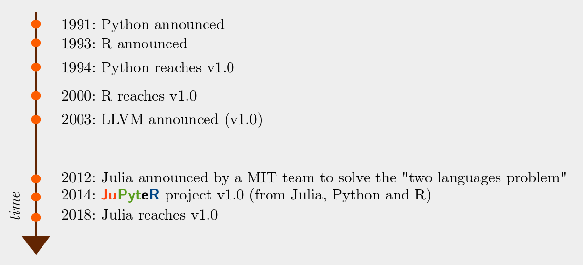
A comparative timeline of R, Python, Julia, LLVM
JIT (Just In Time) compilation:
- R:
compilerlibrary (JIT default in R 3.4) - Python: Numba, PyPy, ...
- Julia: natively, with type inference
Julia is the only language that has been designed for JIT and not trying to be adapted to. Indeed Python, R (but also Matlab..) design makes it really hard to use JIT with these languages and limits its use to a subset of the language, with all the problems of compatibilities that it derives.
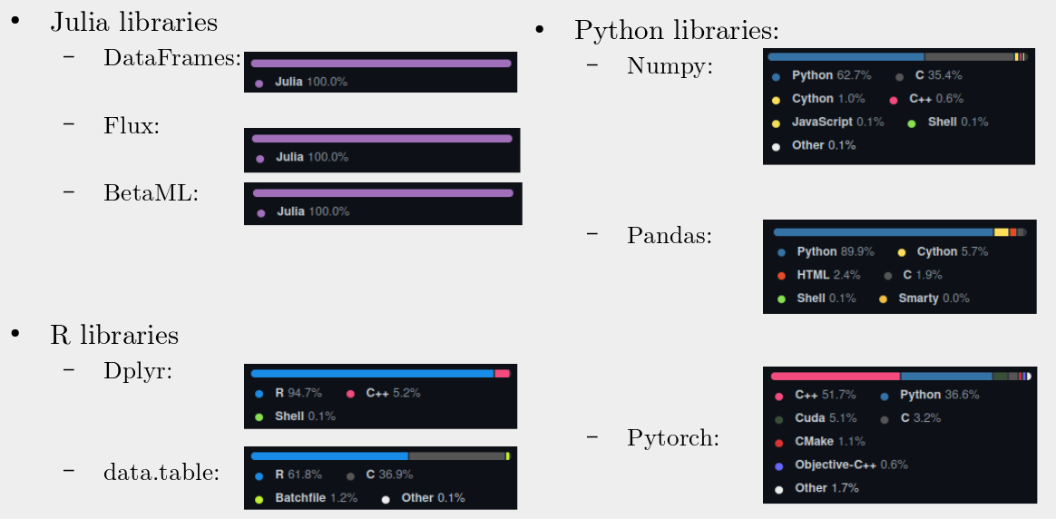
The following figure shows the language used to code some of the most important scientific libraries in these languages, as reported by GitHub. We can see that when performances matter, except for Julia libraries, these projects always rely upon a compiled language. If this is not a problem for a user, it creates a barrier between indeed the user of the library, that is a Python or R programmer, and its developer, that must be proficient in C, Fortran or whatever is the compiled language used. In Julia instead, the user and the developer literally "speak the same language" and collaboration can happen much easier.
Multiple dispatch
As the name implies, multiple dispatch is a programming paradigm where function calls are dispatched at run-time to the actual implementation based not only on the function name but also on the types of all the arguments.
For example:
julia> mysum(a::Number,b::Number) = a+b # Define the first "method" of the mysum function taking parameters a and bmysum (generic function with 1 method)julia> mysum(a::Number,b::Vector) = [a + bi for bi in b] # second method definitionmysum (generic function with 2 methods)julia> mysum(a::Vector,b::Number) = mysum(b,a) # third method definitionmysum (generic function with 3 methods)julia> mysum(a::Vector,b::Vector) = [a[i] + b[i] for i in 1:min(length(a),length(b))] # fourth method definitionmysum (generic function with 4 methods)julia> mysum(10,2) # call the first method12julia> mysum([10,100],2) # call the third method2-element Vector{Int64}: 12 102julia> mysum([10,100],[20,200]) # call the fourth method2-element Vector{Int64}: 30 300
Where the square brackets are to make a list comprehension, a concise way to implement for loops we'll see in the next unit. Note that we don't need to implement mysum ourselves. The default sum already accounts for multiple dispatch and broadcasting, a concept we will see later.
Multiple dispatch can be considered a generalisation of the single argument dispatch system employed in classical object-oriented (OO) languages. To call a function in OO we typically employ a syntax like myobject.foo(argA, argB). But this is syntactically equivalent to foo(myobject,argA,argB), and the call can be dispatched based on the class of myobject, that is of the first argument, but not on the types of argA or argB like in Julia. Multiple dispatch shouldn't be confused with C++-style polymorphism that happens at compile time.
Why multiple dispatch is important ? Firstly, in combination with JIT and for type-stable methods (again, we will see what this means in unit JULIA1), multiple dispatch allows continuing the type inference across the function calls without looking out the type of the arguments at each call, greatly improving performances. Secondly, multiple dispatch improves code composition: when a user introduces a new type, it needs to specify how this new type should handle low-level functionalities. At this point, high-level functionality will work automatically, even if the high-level functionality knew nothing of this new type.
Let's take an example:
julia> X = [1 2 3; 4 5 6] # a matrix2×3 Matrix{Int64}: 1 2 3 4 5 6julia> Y = [[1,2,3] [4,5,6]] # a vector of vectors # Low level function:3×2 Matrix{Int64}: 1 4 2 5 3 6julia> mydivide(x,y) = x/y; # "normal" division (produces a float)julia> mydivide(x::Int64,y::Int64) = x÷y; # so-called "integer" division (truncated)julia> mydivide(x,y::Matrix) = x * y^(-1); # invert matrix yjulia> 11÷3 # 33
In the code above, assume mydivide() is some low-level functionality I implemented relative to integers, floats and matrices. The beauty of multiple dispatch is that with high-level functionalities, I don't need to care about types as long as the low-level functions embedded in these high-level functions work for the arguments I am using. For example, if I have a high-level function foo defined as;
julia> function foo(x,y)
            z = x*y
            mydivide(5,z)
       endfoo (generic function with 1 method)
I can then call it with:
julia> foo(2,3)0julia> foo(3,1.5)1.1111111111111112julia> foo(X,Y)2×2 Matrix{Float64}: 7.12963 -2.96296 -2.96296 1.2963
In all these cases foo will work just because the functionalities that foo uses work with the given argument types.
In conclusion, when introducing a new type, I can care only about the (small) low-level aspects, without having to rebuild the whole Application Programming Interface (API).
Multiple kinds of parallel computation
There is no global interpreter lock in Julia and the programmer is free to use different parallelism paradigms, from the hardware level to distributed computation in High-Performance Computing (HPC) clusters, all using a high-level API:
- Hardware level SIMD (single instruction multiple data), GPU
@simd for i in …CUDA.jlAPI
- Multithreading
Threads.@threads for i in …
- Multiprocessing
addprocs(n, ssh parameters)(on the same machine or on other HPC nodes using SSH tunnelling)@everywhere function foo(arg) …pmap(foo,data)
(details on the last segment of JULIA1 unit.)
Macro and meta-programming
Julia is reflective and allows meta-programming and macros at the level of the Abstract Syntax Tree (AST), that is, when the expressions are already been parsed from the raw source code text. This is more powerful than C-like text-based preprocessing macros as it allows the programmer to hack directly into the AST to change it according to its needs. Perhaps the single more important benefit of this kind of meta-programming is that it brings flexibility in allowing to write very concise library APIs. Let's take the example of Algebraic modelling languages (AML), high-level but specialised computer programming languages for the description and solution of large scale mathematical optimization problems (AMPLL, GAMS,..). Being specialised languages, their syntax is very similar to the mathematical notation of optimization problems, and this allows for a very concise and readable definition of problems in their specific domain (optimization), which is supported by certain language elements. Now, a recent trend is to replace these specialised languages with AML libraries to be used within a more general-purpose language. In languages without meta-programming (like the Pyomo library for Python) this comes at the cost to be forced to use the host language syntax and having to employ a much more verbose syntax. With metaprogramming instead we can allow the library user to write its statements still using a concise, domain-specific way, and it is the macro that will expand this syntax to the one suitable for processing by the hosting language (this is the case of JuMP for Julia)
Other important Julia characteristics
- Extended Unicode support for any identifier and other "syntactic sugar goodies": they allow the code representation of an algorithm to be very close to its math representation, e.g.
x̃₂ ∈ [1,2,π,ℯ]orβ = 2α + 3ℯ^x - Support to user-defined primitive type (need an
Int24type ??).Even basic operators are extendible:+(x,y::Int24) = …. - Linear algebra is built-in:
x' * Y^(-1) - Broadcasting is supported for any function (including user-defined ones):
foo.(args)(note the dot) - Direct interoperability with C and Fortran libraries (
ccall(:foo,foolib,…)) and VERY easy integration with R, Python and other "older" languages - Modern testing and documentation facilities (
Testmodule – in the standard library -,Literate.jl,Documenter.jl, integration with GitHub actions and CodeCov) - Garbage-collection of the memory
- Easy debugging and sample-based profiling
- Git-based package management and light-wise environments for easy replicability. Last but not least. This is a crucial point in scientific programming, and we'll learn more about it already in this introductory lesson.
How to install Julia and git and how to work with them
A preamble on version control software
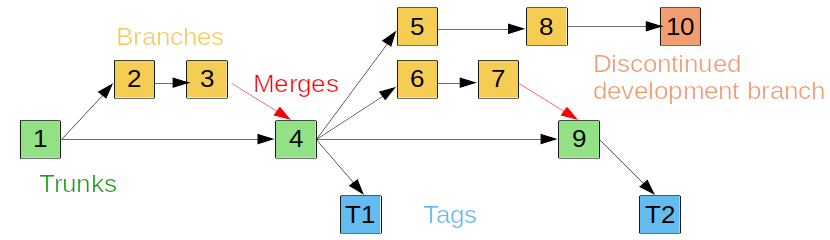
Version control systems are used to keep track of the development of a project and allow easy integration of multiple sub-projects or team contributions. As the figure above shows, they typically allow assigning a name/log entry to a given “screenshot in time” of project development (commits and tags), visualise differences between them, create and merge branches of different development pathways, automatically manage or facilitate resolution of conflicts between versions,...
- First-generation (CVS, SVN,…):
- They were based on a client-server model → the full project (history) is kept in a centralised server and individual users connect and keep on their local pc one specific version
- Second generation (Git, Mercurial, Bazaar,...):
- They adopt a distributed model → each user has the whole copy (including the history) of the project and exchanges its contribution with the other “remote” nodes
- It increases redundancy
- It decreases network load
- It faster operations (many operations – e.g. diff – can be fully done locally)
In particular, Julia packages are git-based, and most of them are hosted (or better, mirrored, as we saw that each node in git - called "remote" - is a full copy of the project) on GitHub, a popular hub of git-based projects.
Set up the environment required for this course
We learn now how to set up Julia itself, VSCode and its Julia plugin (the development environment) and the git client. Please refer to the video for a more visual guide.
Julia (terminal)
Go to https://julialang.org/ → download → 1.7 (or later version) 64 bit installer
- Windows: run with the option "add Julia to path"
- Linux: unzip to
~/lib/julia-1.7.2(or whatever) and symlink~/lib/julia-1.7.2/bin/juliato~/bin/julia1.7with another symlink~/bin/juliapointing to it. This set-up has the advantage that you can have - and run - at the same time multiple versions of Julia. When version 1.8 arrives you can download and unzip it and have the~/bin/julia1.8link with~/bin/juliapointing to it, but you will still have~/bin/julia1.7, and so on for successive versions.
Visual Studio Code
Install Visual Studio Code: https://code.visualstudio.com/ → download → install Note that "Visual Studio" is another product than "Visual Studio Code".
Visual Studio Code Julia extension
From within Visual Studio code, search the extensions: "Julia" (not "Julia insider") Eventually, if for some reason you didn't set up the Julia interpreter in your OS Path, you can set its path in the extension settings.
After installing the Julia extension you can try it by selecting File → New file → Select a language → Julia → type println("Hello World!") followed by SHIFT+ENTER. This should evaluate the command and print "Hello World!" both in the terminal at the bottom and as a hoover on the side of the command.
Git client
While not strictly necessary to work with Julia or for this course (the Julia executable already ships with a minimal git client to manage packages) it is convenient to have installed a full git client and get Visual Studio to recognise it. In Linux just use the package manager to install the version of the git client for your distribution, in Windows download it from https://git-scm.com/download/win and install it by explicitly setting git on the PATH and select to use VSCode. You may need to reboot your system before Visual Studio recognises the git client presence.
A first look at git(hub): a git workflow exercise
We will now go through an exercise to start a new git project on GitHub, "clone" it on our local computer, modify it and "push" our modifications back on the GitHub server.
But before let's note a list of essential git commands:
git clone [url]: "Clone" an existing repository locally, that it transfers the project files of the current and all previous versions (i.e. the full history of the project)git init(inside a given directory): Tell git to treat the current directory as a (new) git projectgit add [file]: Add a file to the git project (the project must already exist either because we rangit initor we cloned it from a remote repository)git commit -a -m “[message]”: Commit your work, i.e. save as a specific version in the project. This "version" will have an id, will appear in the git logs and can be "tagged" to be easily retrieved- Branches:
git branch: See all the "branches" of a project, the parallel development histories associated with itgit branch [branchname]: Create a new branchgit checkout [branchname]: Switch to an existing branchgit merge [branchname]: Merge the named branch to the current onegit branch -d [branchname]: Delete a local branch
- Working with remotes:
git fetch: Fetch content from a remote repository (without attempting to update the local repository)git pull: Fetch and try to merge locally from a remote repositorygit push: Push the data to a remote repositorygit remote: List all the remote repositories (when we clone from GitHub we have that remote listed by default asorigin)
- Information:
git status: Get the status of the current repositorygit log: Get git logsgit diff:See diff with HEADgit diff [commithash1] [commithash2]See diff between any arbitrary commit(s)
Further information specific on Git can fe found on:
- Git tutorials (shorts):
- https://git-scm.com/docs/gittutorial
- https://thenewstack.io/tutorial-git-for-absolutely-everyone
- Git book (long):
- https://git-scm.com/book
Let's now create, as an exercise, our first git repository, clone locally, make some edits and push it back on GitHub. Again, if you are lost following the text, watch the video above for a visual guide.
First register or sign in on github.com and add a new repository, for example, "testGit". Attention to the capital letters, they matter, and don't use spaces in the project name. In the project creation form, select the options to add a readme file, a gitignore (for Julia) and a licence of your choice.
We are now ready to clone the repository locally using Visual Code Studio, either using an automatic way or a more "manual" approach. In the first case:
- From within Visual Studio Code, type
CTRL+SHIFT+Pto open the command palette and search forgit:clone - Select "Clone from GitHub"
- If needed, provide the required authorisation
- Select a repository
- Select the local folder where to clone the repository
- Optionally open or add the newly cloned repository to the workspace
For the manual way:
- Open a new "git bash" terminal using "new terminal" and then the "plus" symbol
- Type in the terminal
git clone https://github.com/[YOUR GITHUB USERNAME]/testGit.git - Open the folder that should be located on
This PC>OS (C:)>Users>[Your name]>testGit
We can now do some basic work locally and push it back on GitHub:
- Using the VS Code explorer, add a file "test.jl"
- On that file write
println("Hello World!")and save - Edit the README.md file (type what you want)
- If not already open, open a new "git bash" terminal using "new terminal" and then the "plus" symbol
- Type in the terminal
git status. It should return to you that there is a "modified" file under "Changes not staged for commit" and a file (ourtest.jl) under "Untracked files" - Type in the terminal
git add test.jlfollowed bygit statusagain. Nowtest.jlshould be under "New file" - If you never used git on this pc, type this (this is needed only once to tell git who you are):
- git config –global user.email "your@email.com"
- git config –global user.name "Your Name"
- Type in the terminal
git commit -a, add a message for the log, pressCTR+XandYto confirm: you created a new commit, a permanent "version" of your project to which you can always "go back" whenever needed - Type
git pushand follow the online instruction to authorise: the commit, that up to now was still only on your local machine, is "transferred" to the remote node, GitHub in this case
If you go or refresh your browser on https://github.com/[YOUR GITHUB USERNAME]/testGit.git you should now visualise the modifications you made to the repository. Finally, let's try some basic branch workflow.
- Edit the file
test.jlto add some text on the lines 4, 7 and 9, save and commit as before - Type in the terminal
git branch tempto create a new branch named temp andgit checkout tempto move on that specific branch - Now edit
test.jlon line 9, save and commit again - Let's go back to the
main(default) branch withgit checkout main. Note how the modifications you made on point3"seem" to have disappeared
Note that until a few years ago the default branch name on all git systems was "master". Most old projects still use that name for their default branch.
- Edit
test.jlon line 5, save and commit - Type in the terminal
git diff main tempto see the differences between the two branches - Type in the terminal
git branchto display all the available branches. The current one is highlighted with a star. Be sure it ismain - Type in the terminal
git merge tempto merge the work you have done in the branchtemp(the modifications on line 9) in the currentmainbranch - Type in the terminal
git logto retrieve a log of the commits you made - Type in the terminal
git pushto push the modifications to the remote( GitHub) - Type in the terminal
git branch -d tempto remove the nolongerneededtempbranch
While git has many more commands and options, the commands above are enough to start becoming operational with git. Again, I suggest cloning the git repository of this course (git clone https://github.com/sylvaticus/SPMLJ.git) and playing with the commands by yourself.
Julia modules, packages and environments
As anticipated, we start our study of Julia from its modules, packages and environments rather than its syntax.
Modules and packages
Modules are some logical grouping of program functionalities. Functions, custom-defined types, constants and other objects can be grouped in modules. Modules help in keeping the "namespace", the set of the names from which the various objects of the program can be accessed, "clean", so that we can refer to molule1.foo and module2.foo objects separately.
Packages are just modules, a single module with the same name of the package, plus some "metadata" that facilitates its discovery and interplay with other packages – where I find it, which version I am using, which other packages – and versions – this module depends from, etc.
A typical module would look like this:
module ModuleName
export myObjects # functions, structs, and other objects that will be directly available once `using ModuleName` is typed
# [...module code...]
end
Module names are customary starting with a capital letter and the module content is usually not indented. Modules can be entered in the REPL as normal Julia code or in a script that is imported with include("file.jl").
include causes the included code to be evaluated at the global scope of the module where the include call occurs.
Organise your code as the same code is never included multiple times or it will likely cause problems, as in the definition of structures or constants
There is no connection between a given file and a given module as in other languages, so the logical structure of a program can be decoupled from its actual division in files. For example, one file could contain multiple modules. The typical pattern is to define a new module, and then include the various files that compose the module, depending on the organisation we want to give to the module.
All modules are children of the module Main, the default module for global objects in Julia, and each module defines its own set of global names.
Modules can be used with one of the following commands:
using pkgOrModule
import pkg # `import module` would be useless
import pkgOrModule: X,Y,Z
The first command above brings into scope only the module or package objects explicitly named in export, the second, while loading the package into memory it doesn't bring any objects into scope (we need then to refer to any module's object as module.object), finally with the third command we chose the objects to bring into scope at import time rather than when we wrote the module or package.
using and import, when they are followed with either Main.x or .x, look for a module already loaded and bring it and its exported objects into scope (for import only those explicitly specified). Otherwise, they do a completely different job: they expect a package, and the package system lookups for the correct version of the module x embedded inside package x, it loads it, and it brings it and its exported objects into scope (again, for import x only those explicitly specified).
While modules can have submodules (childs), this is rarely employed in Julia. In such cases use a chained dot syntax to refer to them, e.g. module1.childb.subchild3.
Package manager
Julia packages are essentially git repositories – not necessarily hosted on github.com - that include a module plus some metadata in a Project.toml file and some other elements like a test script, a subfolder "doc" from which the package documentation is built, etc. The commands of the package manager shown below issue, under the hood, various git commands.
Some useful package commands:
status: Retrieves a list with names and versions of locally installed packagesupdate: Updates the local index of packages and all the local packages to the latest versionadd myPkg: Automatically downloads and installs a packagerm myPkg: Removes a package and all its dependent packages that have been installed automatically only for itadd pkgName#master: Checkouts the master branch of a packageadd pkgName#branchName: Checkout a specific branchadd git@github.com:userName/pkgName.jl.git: Checkout a non-registered pkgfree pkgName: Return to the "standard" latest compatible released version of a package
To issue a package command first type ] in the REPL to enter a special "package mode" and then enter the command. Alternatively, in a script we can first import Pkg and then run the commands as Pkg.command(options).
Note that pretty uniquely within package managers, Julia packages, when providing compatible versions of packages they depend on, must specify both the lower but also the upper range.
If you wish to develop a Julia package you can refer to this tutorial.
Environments
Packages themselves are downloaded, "installed" (precompiled) and stored in a centralised user directory (e.g. /home/[username]/.julia in Linux). Each project can (should!) have its own "environment", as this wouldn't consume any more resources, because multiple projects having the same version of a package as a dependency, will just share it.
Environments in Julia are really simple and "light", as the "environment" is composed just of a couple of small, automatically managed text files: Project.toml file that lists the packages directly used in the project (and optionally - but mandatorily for registered packages - their version ranges), and Manifest.toml, that lists all the packages and sub-packages used in the project and their exact versions. The environment refers to the directory where these two files live.
These files are automatically updated when you add, update or make any other package operation within that environment. Providing them to the "customer", to the journal editor, or to yourself 20 years later, will guarantee that your results are still replicable (of course, together with the source code, the program inputs, and, if your program includes some stochastic parts, conditional to the adoption of a fixed seed for the random number generator).
Your recipient will just need then to type something like the code below to retrieve exactly the same set of packages you used to run your program:
cd(@__DIR__)
using Pkg
Pkg.activate(".")
Pkg.instantiate()
The first line sets the current directory to those of the *.jl file in which the command is present, the third line activates the environment at the current directory and the fourth line reads the content of the Manifest.toml file in the environment directory and take care to download and reinstall all the packages at the exactly given versions.
Attention to this difference: the current directory is the path that serves as a reference when you interact with the operating system for files input/output, for example, to read a Comma Separated File or to save a plot image. The environment is the directory where the associated Metadata.toml and Project.toml files listing all the dependencies reside. The two directories can be the same but also be different.