EXERCISE 2.1: Fitting the growth of French forests
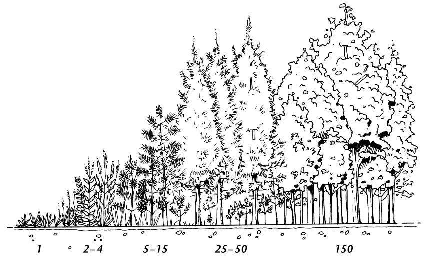
How fast are French forests growing? How much timber can they provide in one hectare? Surely forests provide multiple ecosystem services, but in this (simplified) exercise we focus on the above questions by looking at the so-called "raw data" provided by the French National Forest Inventory, both in terms of individual trees and in terms of inventoried plots, to fit a generic growth model of the forest stands in terms of volumes with respect to the age of the trees.
Skills employed:
- download and import data from internet
- wrangle tabular data: compute new columns (fields) based on existing one, filter rows (records), join tables
- fit a generic model (curve) with data
Instructions
If you have already cloned or downloaded the whole course repository the folder with the exercise is on [REPOSITORY_ROOT]/lessonsMaterial/02_JULIA2/forestExercise. Otherwise download a zip of just that folder here.
In the folder you will find the file forestExercise.jl containing the julia file that you will have to complete to implement and run the model (follow the instructions on that file). In that folder you will also find the Manifest.toml file. The proposal of resolution below has been tested with the environment defined by that file. If you are stuck and you don't want to lookup to the resolution above you can also ask for help in the forum at the bottom of this page. Good luck!
Resolution
Click "ONE POSSIBLE SOLUTION" to get access to (one possible) solution for each part of the code that you are asked to implement.
1) Setting up the environment...
Start by setting the working directory to the directory of this file and activate it. If you have the provided Manifest.toml file in the directory, just run Pkg.instantiate(), otherwise manually add the packages Pipe, HTTP, CSV, DataFrames, LsqFit, StatsPlots.
ONE POSSIBLE SOLUTION
cd(@__DIR__)
using Pkg
Pkg.activate(".")
# If using a Julia version different than 1.10 please uncomment and run the following line (reproductibility guarantee will hower be lost)
# Pkg.resolve()
Pkg.instantiate()
using Random
Random.seed!(123)
2) Load the packages
Load the packages Pipe, HTTP, CSV, DataFrames, LsqFit, StatsPlots
ONE POSSIBLE SOLUTION
using Pipe, HTTP, CSV, DataFrames, LsqFit, StatsPlots3) Load the data
Load from internet or from local files the following data:
ltURL     = "https://github.com/sylvaticus/IntroSPMLJuliaCourse/blob/main/lessonsMaterial/02_JULIA2/forestExercise/data/arbres_foret_2012.csv?raw=true" # live individual trees data
dtURL     = "https://github.com/sylvaticus/IntroSPMLJuliaCourse/blob/main/lessonsMaterial/02_JULIA2/forestExercise/data/arbres_morts_foret_2012.csv?raw=true" # dead individual trees data
pointsURL = "https://github.com/sylvaticus/IntroSPMLJuliaCourse/blob/main/lessonsMaterial/02_JULIA2/forestExercise/data/placettes_foret_2012.csv?raw=true" # plot level data
docURL    = "https://github.com/sylvaticus/IntroSPMLJuliaCourse/blob/main/lessonsMaterial/02_JULIA2/forestExercise/data/documentation_2012.csv?raw=true" # optional, needed for the species label
If you have choosen to download the data from internet, you can make for each of the dataset a @pipe macro starting with HTTP.get(URL).body, continuing the pipe with CSV.File(_) and end the pipe with a DataFrame object.
ONE POSSIBLE SOLUTION
lt     = @pipe HTTP.get(ltURL).body     |> CSV.File(_) |> DataFrame
dt     = @pipe HTTP.get(dtURL).body     |> CSV.File(_) |> DataFrame
points = @pipe HTTP.get(pointsURL).body |> CSV.File(_) |> DataFrame
doc    = @pipe HTTP.get(docURL).body    |> CSV.File(_) |> DataFrame

# Or import from local...
lt     = CSV.read("data/arbres_foret_2012.csv",DataFrame)
dt     = CSV.read("data/arbres_morts_foret_2012.csv",DataFrame)
points = CSV.read("data/placettes_foret_2012.csv",DataFrame)
doc    = CSV.read("data/documentation_2012.csv",DataFrame)
4) Filter out unused information
These datasets have many variable we are not using in this exercise. Out of all the variables, select only for the lt and dt dataframes the columns idp (pixel id), c13 (circumference at 1.30 meters) and v (tree's volume). Then vertical concatenate the two dataset in an overall trees dataset. For the points dataset, select only the variables idp (pixel id), esspre (code of the main forest species in the stand) and cac (age class).
ONE POSSIBLE SOLUTION
lt     = lt[:,["idp","c13","v"]]
dt     = dt[:,["idp","c13","v"]]
trees  = vcat(lt,dt)
points = points[:,["idp","esspre","cac"]]
5) Compute the timber volumes per hectare
As the French inventory system is based on a concentric sample method (small trees are sampled on a small area (6 metres radius), intermediate trees on a concentric area of 9 metres and only large trees (with a circonference larger than 117.5 cm) are sampled on a concentric area of 15 metres of radius), define the following function to compute the contribution of each tree to the volume per hectare:
"""
    vHaContribution(volume,circonference)

Return the contribution in terms of m³/ha of the tree.

The French inventory system is based on a concentric sample method: small trees are sampled on a small area (6 metres radius), intermediate trees on a concentric area of 9 metres and only large trees (with a circonference larger than 117.5 cm) are sampled on a concentric area of 15 metres of radius.
This function normalise the contribution of each tree to m³/ha.
"""
function vHaContribution(v,c13)
    if c13 < 70.5
        return v/(6^2*pi/(100*100))
    elseif c13 < 117.5
        return v/(9^2*pi/(100*100))
    else
        return v/(15^2*pi/(100*100))
    end
end
Use the above function to compute trees.vHa based on trees.v and trees.c13.
ONE POSSIBLE SOLUTION
trees.vHa = vHaContribution.(trees.v,trees.c13)6) Aggregate trees data
Aggregate the trees dataframe by the idp column to retrieve the sum of vHa and the number of trees for each point, calling these two columns vHa and ntrees.
ONE POSSIBLE SOLUTION
pointsVols = combine(groupby(trees,["idp"]) , "vHa" => sum => "vHa", nrow => "ntrees")7) Join datasets
Join the output of the previous step (the trees dataframe aggregated "by point") with the original points dataframe using the column idp.
ONE POSSIBLE SOLUTION
points = innerjoin(points,pointsVols,on="idp")8) Filter data
Use boolean selection to apply the following filters:
filter_nTrees           = points.ntrees .> 5 # we skip points with few trees
filter_IHaveAgeClass    = .! in.(points.cac,Ref(["AA","NR"]))
filter_IHaveMainSpecies = .! ismissing.(points.esspre)
filter_overall          = filter_nTrees .&& filter_IHaveAgeClass .&& filter_IHaveMainSpecies
ONE POSSIBLE SOLUTION
points = points[filter_overall,:] 9) Compute the age class
Run the following command to parse the age class (originally as a string indicating the 5-ages group) to an integer and compute the mid-range of the class in years. For example, class "02" will become 7.5 years.
points.cac = (parse.(Int64,points.cac) .- 1 ) .* 5 .+ 2.510) Define the model to fit
Define the following logistic model of the growth relation with respect to the age with 3 parameters and make its vectorised form:
logisticModel(age,parameters) = parameters[1]/(1+exp(-parameters[2] * (age-parameters[3]) ))
logisticModelVec(age,parameters) = # .... complete here
ONE POSSIBLE SOLUTION
logisticModelVec(age,parameters) = logisticModel.(age,Ref(parameters))11) Set the initial values for the parameters to fit
Set initialParameters to 1000,0.05 and 50 respectivelly.
ONE POSSIBLE SOLUTION
initialParameters = [1000,0.05,50] #max growth; growth rate, mid age12) Fit the model
Perform the fitting of the model using the function curve_fit(model,X,Y,initial parameters) and obtain the fitted parameter fitobject.param
ONE POSSIBLE SOLUTION
fitobject         = curve_fit(logisticModelVec, points.cac, points.vHa, initialParameters)
fitparams         = fitobject.param
13) Compute the errors
Compute the standard error for each estimated parameter and the confidence interval at 10% significance level
ONE POSSIBLE SOLUTION
sigma            = stderror(fitobject)
confidence_inter = confidence_interval(fitobject, 0.1) # 10% significance level
14) Plot fitted model
Plot a chart of fitted (y) by stand age (x) (i.e. the logisticModel with the given parameters)
ONE POSSIBLE SOLUTION
x = 0:maximum(points.cac)*1.5
plot(x->logisticModel(x,fitparams),0,maximum(x), label= "Fitted vols", legend=:topleft)
15) Add the observations to the plot
Add to the plot a scatter chart of the actual observed VHa
ONE POSSIBLE SOLUTION
plot!(points.cac, points.vHa, seriestype=:scatter, label = "Obs vHa")16) [OPTIONAL] Differentiate the model per tree specie
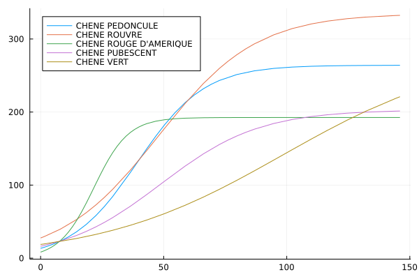
Look at the growth curves of individual species. Try to perform the above analysis for individual species, for example plot the fitted curves for the 5 most common species
ONE POSSIBLE SOLUTION
speciesCount = combine(groupby(points, :esspre), nrow => :count)
sort!(speciesCount,"count",rev=true)

spLabel        = doc[doc.donnee .== "ESSPRE",:]
spLabel.spCode = parse.(Int64,spLabel.code)
speciesCount = leftjoin(speciesCount,spLabel, on="esspre" => "spCode")


# plot the 5 main species separately
for (i,sp) in enumerate(speciesCount[1:5,"esspre"])
    local fitobject, fitparams, x
    spLabel    = speciesCount[i,"libelle"]
    pointsSp   = points[points.esspre .== sp, : ]
    fitobject  = curve_fit(logisticModelVec, pointsSp.cac, pointsSp.vHa, initialParameters)
    fitparams  = fitobject.param
    x = 0:maximum(points.cac)*1.5
    println(i)
    println(sp)
    println(fitparams)
    if i == 1
        myplot = plot(x->logisticModel(x,fitparams),0,maximum(x), label= spLabel, legend=:topleft)
    else
        myplot = plot!(x->logisticModel(x,fitparams),0,maximum(x), label= spLabel, legend=:topleft)
    end
    display(myplot)
end