EXERCISE 3.1: Breast cancer diagnosis using the perceptron algorithm
In this problem we are given a dataset containing real world characteristics of observed breast cancer (size, pattern,..) together with the associated diagnosis in terms of malignity or benignity of the cancer. Our task is to build a linear classifier using the perceptron algorithm that we studied and train it in order to make diagnosis based on the cancer characteristics.
Skills employed:
- download and import data from internet
- implement the training function of a perceptron algorithm
- use the BetaML
partition,crossValidationandaccuracyfunctions
Instructions
If you have already cloned or downloaded the whole course repository the folder with the exercise is on [REPOSITORY_ROOT]/lessonsMaterial/03_ML1/BreastCancerDiagnosisWithPerceptron. Otherwise download a zip of just that folder here.
In the folder you will find the file BreastCancerDiagnosisWithPerceptron.jl containing the Julia file that you will have to complete in order to implement and run it (follow the instructions on that file). In that folder you will also find the Manifest.toml file. The proposal of resolution below has been tested with the environment defined by that file. If you are stuck and you don't want to lookup to the resolution above you can also ask for help in the forum at the bottom of this page. Good luck!
Resolution
Click "ONE POSSIBLE SOLUTION" to get access to (one possible) solution for each part of the code that you are asked to implement.
1) Setting up the environment...
Start by setting the working directory to the directory of this file and activate it. If you have the provided Manifest.toml file in the directory, just run Pkg.instantiate(), otherwise manually add the packages Pipe, HTTP, StatsPlots and BetaML.
ONE POSSIBLE SOLUTION
cd(@__DIR__)
using Pkg
Pkg.activate(".")
# If using a Julia version different than 1.10 please uncomment and run the following line (reproductibility guarantee will hower be lost)
# Pkg.resolve()
Pkg.instantiate()
using Random
Random.seed!(123)
2) Load the packages
Load the packages Statistics, DelimitedFiles, LinearAlgebra, Pipe, HTTP, StatsPlots, BetaML
ONE POSSIBLE SOLUTION
using Statistics, DelimitedFiles, LinearAlgebra, HTTP, StatsPlots, BetaML
import Pipe:@pipe
3) Load the data
Load from internet or from localfile the input data and shuffle its rows (records):
dataURL = "https://raw.githubusercontent.com/sylvaticus/IntroSPMLJuliaCourse/main/lessonsMaterial/03_ML1/BreastCancerDiagnosisWithPerceptron/data/wdbc.data.csv"Source: Breast Cancer Wisconsin (Diagnostic) Data Set, UCI Machine Learning Repository
ONE POSSIBLE SOLUTION
data    = @pipe HTTP.get(dataURL).body |> readdlm(_,',')
nR      = size(data,1)
data    = data[shuffle(1:nR),:]
4) Map the data to (X,y)
The data you have loaded contains the actual diagnosis for the cancer in the second column, coded with a string "B" for "Benign" and "M" for "Malign", and the characteristics of the cancer foir the next 30 columns. Save the diagnosis to the vector y, coding malign cancers with 1 and benign cancers with -1 Save the characteristics to the feature matrix X (and be sure it is made of Float64)
ONE POSSIBLE SOLUTION
y       = map( x -> x == "M" ? 1 : -1,  data[:,2])
X       = convert(Matrix{Float64},data[:,3:end])
nD      = size(X,2)
5) (this task is provided) Plot the data and the classifier
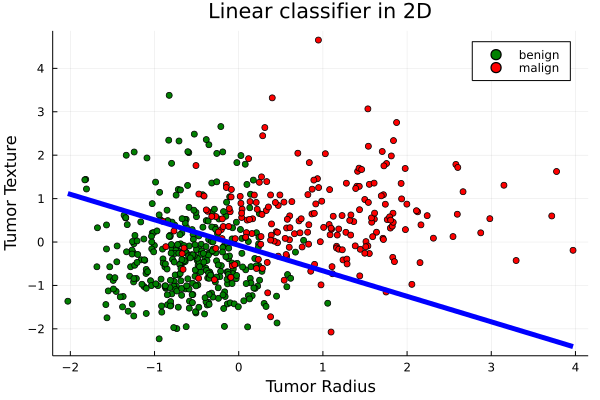
Plot the first 2 attributes of training points and define the function plot2DClassifierWithData()
colors = [y == 1 ? "red" : "green" for y in y]
labels = [y == 1 ? "malign" : "benign" for y in y]
scatter(X[:,1],X[:,2], colour=colors, title="Classified tumors",xlabel="Tumor Radius", ylabel="Tumor Texture", group=labels)

function plot2DClassifierWithData(X,y,θ;d1=1,d2=2,origin=false,xlabel="Dimx: $(d1)",ylabel="Dimy: $(d2)")
    nR    = size(X,1)
    X     = hcat(ones(nR),X)
    X     = fit!(Scaler(),X) # for visualisation
    d1    += 1
    d2    += 1
    colors = [y == 1 ? "red" : "green" for y in y]
    labels = [y == 1 ? "malign" : "benign" for y in y]
    minD1,maxD1 = extrema(X[:,d1])
    minD2,maxD2 = extrema(X[:,d2])
    myplot = scatter(X[:,d1],X[:,d2], colour=colors, title="Linear classifier in 2D",xlabel=xlabel, ylabel=ylabel, group=labels)
    d2Class(x) = -θ[1]/θ[d2] -x * θ[d1]/θ[d2]
    if θ[d2] == 0
        vline!([0], color= "blue",label="",linewidth=5)
    else
        plot!(d2Class,minD1,maxD1, color= "blue",label="",linewidth=5)
    end
    display(myplot)
end
6) (provided) Define the Model and training options
abstract type SupervisedModel end
abstract type TrainingOptions end

mutable struct Perceptron <: SupervisedModel
    θ::Vector{Float64}
end

mutable struct PerceptronTrainingOptions <: TrainingOptions
    epochs::Int64
    verbose::Bool
    shuffle::Bool
    function PerceptronTrainingOptions(;epochs=1,verbose=false,shuffle=false)
        return new(epochs,verbose,shuffle)
    end
end
7) (provided) Implement the functions predict() and update()
function predict(model::Perceptron,x::AbstractVector)
    x = vcat(1.0,x)
    x' * model.θ > eps() ? (return 1) : (return -1)
end

function predict(model::Perceptron,X::AbstractMatrix)
    return [predict(model,r) for r in eachrow(X)]
end

function update!(model::Perceptron,X::Vector,y)
    X       = vcat(1.0,X)
    model.θ = model.θ .+ y .* X
    return model.θ
end
8) Implement the training function
Implement the function train!(model::Perceptron,X,y,ops=PerceptronTrainingOptions()::TrainingOptions)
Compared to the function we saw in the 0302-perceptron.jl file, add, if you wish, a counter to eventually return early if there are no more errors in an epoch (i.e., all points are correctly classified)
function train!(model::Perceptron,X,y,ops=PerceptronTrainingOptions()::TrainingOptions)
    #...
    for t in 1:epochs
        #...
        if ops.shuffle
           #...
        end
        for n in 1:nR
           #...
        end
        #...
    end
    #...
    return model.θ
end
ONE POSSIBLE SOLUTION
function train!(model::Perceptron,X,y,ops=PerceptronTrainingOptions()::TrainingOptions)
    epochs  = ops.epochs
    verbose = ops.verbose
    (nR,nD) = size(X)
    nD += 1
    for t in 1:epochs
        errors = 0
        errorsPerEpoch = 0
        if ops.shuffle   # more efficient !
          idx = shuffle(1:nR)
          X = X[idx,:]
          y = y[idx]
        end
        for n in 1:nR
            if verbose
                println("$n: X[n,:] \t θ: $(model.θ)")
            end
            if  predict(model,X[n,:]) != y[n]
                errors += 1
                errorsPerEpoch += 1
                update!(model,X[n,:],y[n])
                if verbose
                    println("**update! New theta: $(model.θ)")
                end
            end
        end
        if verbose
            println("Epoch $t errors: $errors")
        end
        if errorsPerEpoch == 0
            return model.θ
        end
    end
    return model.θ
end
9) Train, predict and evaluate the model
Instanziate a Perceptron object with a parameter vector of nD+1 zeros and a PerceptronTrainingOption object with 5 epochs and shuffling, use the options to train the model on the whole dataset, compute the model predictions and the accuracy relative to the whole sample.
m   = Perceptron(zeros(size(X,2)+1))
ops = #...
train!(m,X,y,ops)
plot2DClassifierWithData(X,y,m.θ,d1=1,d2=2,xlabel="Tumor Radius", ylabel="Tumor Texture")
ŷ           = #...
inSampleAcc = accuracy(#= ... =#) # 0.91
ONE POSSIBLE SOLUTION
ops = PerceptronTrainingOptions(epochs=5,shuffle=true)
ŷ           = predict(m,X)
inSampleAcc = accuracy(ŷ,y) # 0.91
10) Partition the data
Partition the data in (xtrain,xtest) and (ytrain,ytest) keeping 65% of the data for training and reserving 35% for testing
((xtrain,xtest),(ytrain,ytest)) = partition(#=...=#)ONE POSSIBLE SOLUTION
((xtrain,xtest),(ytrain,ytest)) = partition([X,y],[0.65,0.35])11) Implement cross-validation
Using a 10-folds cross-validation strategy, find the best hyperparameters within the following ranges :
sampler = KFold(#=...=#)

epochsSet  = 1:5:150
shuffleSet = [false,true]

bestE       = 0
bestShuffle = false
bestAcc     = 0.0

accuraciesNonShuffle = []
accuraciesShuffle    = []

for e in epochsSet, s in shuffleSet
    global bestE, bestShuffle, bestAcc, accuraciesNonShuffle, accuraciesShuffle
    local acc
    local ops  = PerceptronTrainingOptions(#=...=#)
    (acc,_)    = cross_validation([xtrain,ytrain],sampler) do trainData,valData,rng
                    (xtrain,ytrain) = trainData; (xval,yval) = valData
                    m               = Perceptron(zeros(size(xtrain,2)+1))
                    train!(#=...=#)
                    ŷval            = predict(#=...=#)
                    valAccuracy     = accuracy(#=...=#)
                    return valAccuracy
                end
    if acc > bestAcc
        bestAcc     = acc
        bestE       = e
        bestShuffle = s
    end
    if s
        push!(accuraciesShuffle,acc)
    else
        push!(accuraciesNonShuffle,acc)
    end
end
ONE POSSIBLE SOLUTION
sampler = KFold(nsplits=10)
local ops  = PerceptronTrainingOptions(epochs=e,shuffle=s)
(acc,_)    = cross_validation([xtrain,ytrain],sampler) do trainData,valData,rng
                (xtrain,ytrain) = trainData; (xval,yval) = valData
                m               = Perceptron(zeros(size(xtrain,2)+1))
                train!(m,xtrain,ytrain,ops)
                ŷval            = predict(m,xval)
                valAccuracy     = accuracy(ŷval,yval)
                return valAccuracy
            end
bestAcc # 0.91
bestE
bestShuffle
plot(epochsSet,accuraciesNonShuffle,label="Val accuracy without shuffling", legend=:bottomright)
plot!(epochsSet,accuraciesShuffle, label="Val accuracy with shuffling")12) Train, predict and evaluate the "optimal" model
Using the "best" hyperparameters found in the previous step, instantiate a new model and options, train the model using (xtrain,ytrain), make your predicitons for the testing features (xtest) and compute your output accuracy compared with those of the true ytest (use the BetaML function accuracy).
ops = PerceptronTrainingOptions(#=...=#)
m   = Perceptron(zeros(size(xtest,2)+1))
train!(#=...=#)
ŷtest           = predict(#=...=#)
testAccuracy    = accuracy(#=...=#) # 0.89
ONE POSSIBLE SOLUTION
ops = PerceptronTrainingOptions(epochs=bestE,shuffle=bestShuffle)
m   = Perceptron(zeros(size(xtest,2)+1))
train!(m,xtrain,ytrain,ops)
ŷtest           = predict(m,xtest)
testAccuracy    = accuracy(ŷtest,ytest) # 0.89
plot2DClassifierWithData(xtest,ytest,m.θ,xlabel="Tumor Radius", ylabel="Tumor Texture")
plot2DClassifierWithData(xtest,ytest,m.θ,d1=3,d2=4)13) (optional) Use scaled data
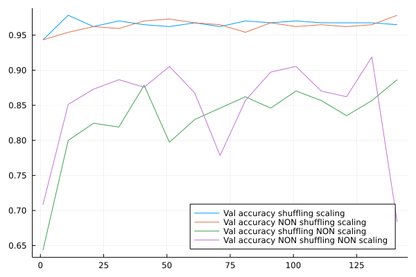
Optionally, add a scaling passage to the workflow and test it with cross-validation if it improves the accuracy
epochsSet  = 1:10:150
shuffleSet = [false,true]
scalingSet = [false,true]

bestE       = 0
bestShuffle = false
bestScaling = false
bestAcc     = 0.0

accNShuffleNSc = Float64[]
accNShuffleSc  = Float64[]
accShuffleNSc  = Float64[]
accShuffleSc   = Float64[]

xtrainsc = fit!(Scaler(),xtrain)

for e in epochsSet, s in shuffleSet, sc in scalingSet
    global bestE, bestShuffle, bestAcc, accNShuffleNSc, accNShuffleSc, accShuffleNSc, accShuffleSc
    local acc
    local ops  = PerceptronTrainingOptions(#=...=#)
    xtrainsc= copy(xtrain)
    if(sc)
        xtraintouse = fit!(Scaler(),xtrain)
    else
        xtraintouse = copy(xtrain)
    end
    (acc,_)    = cross_validation([xtraintouse,ytrain],sampler) do trainData,valData,rng
                    #...
                    return valAccuracy
                end
    if acc > bestAcc
        bestAcc     = acc
        bestE       = e
        bestShuffle = s
        bestScaling = sc
    end
    if s && sc
        push!(accShuffleSc,acc)
    elseif  s && !sc
        push!(accShuffleNSc,acc)
    elseif  !s && sc
        push!(accNShuffleSc,acc)
    elseif  !s && !sc
        push!(accNShuffleNSc,acc)
    else
        @error "Something wrong here"
    end
end
ONE POSSIBLE SOLUTION
local ops  = PerceptronTrainingOptions(epochs=e,shuffle=s)
(acc,_)    = cross_validation([xtrainsc,ytrain],sampler) do trainData,valData,rng
                (xtrain,ytrain) = trainData; (xval,yval) = valData
                m               = Perceptron(zeros(size(xtrain,2)+1))
                train!(m,xtrain,ytrain,ops)
                ŷval            = predict(m,xval)
                valAccuracy     = accuracy(ŷval,yval)
                return valAccuracy
            end
bestAcc # 0.97
bestE
bestShuffle
bestScaling
plot(epochsSet,accShuffleSc,label="Val accuracy shuffling scaling", legend=:bottomright)
plot!(epochsSet,accNShuffleSc,label="Val accuracy NON shuffling scaling", legend=:bottomright)
plot!(epochsSet,accShuffleNSc,label="Val accuracy shuffling NON scaling", legend=:bottomright)
plot!(epochsSet,accNShuffleNSc,label="Val accuracy NON shuffling NON scaling", legend=:bottomright)
ops = PerceptronTrainingOptions(#=...=#)
m = Perceptron(#=...=#)
if bestScaling
train!(m,fit!(Scaler()xtrain),ytrain,ops)
ŷtest = predict(m,fit!(Scaler,xtest))
else
train!(m,xtrain,ytrain,ops)
ŷtest = predict(m,xtest)
end
testAccuracy = accuracy(#=...=#) # 0.96ONE POSSIBLE SOLUTION
ops = PerceptronTrainingOptions(epochs=bestE,shuffle=bestShuffle)
m   = Perceptron(zeros(size(xtest,2)+1))
testAccuracy    = accuracy(ŷtest,ytest) #
plot2DClassifierWithData(xtest,ytest,m.θ,xlabel="Tumor Radius", ylabel="Tumor Texture")