EXERCISE 2.2: The profit maximisation problem
You are the decision-maker of a production unit (here a logging company) and have a set of possible activities to undergo. How do you choose the activities that lead to a maximisation of the unit's profit?
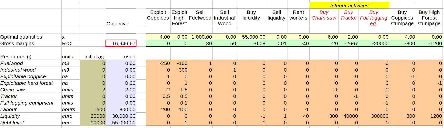
The objective of this problem is hence to find the optimal level of activities to maximise the company profit, given (a) the profitability (gross margin) of each activity, (b) the resources available to the company and (c) the matrix of technical coefficients that link each activity to the resources required (positive coefficient) or provided (negative coefficient) by that specific activity.
The problem is the same as those in the SpreadSheet file "Optimal production mix.ods" (available in the data folder) and can be solved in LibreOffice by using the "Solver tool" as indicated in that file. You can use it to check your results.
Skills employed:
- download and import data from internet
- define, solve and retriever optimal values of an optimisation problem using the JuMP algebraic modelling language
Instructions
If you have already cloned or downloaded the whole course repository the folder with the exercise is on [REPOSITORY_ROOT]/lessonsMaterial/02_JULIA2/loggingOptimisation. Otherwise download a zip of just that folder here.
In the folder you will find the file loggingOptimisation.jl containing the julia file that you will have to complete to implement and run the model (follow the instructions on that file). In that folder you will also find the Manifest.toml file. The proposal of resolution below has been tested with the environment defined by that file. If you are stuck and you don't want to lookup to the resolution above you can also ask for help in the forum at the bottom of this page. Good luck!
Resolution
Click "ONE POSSIBLE SOLUTION" to get access to (one possible) solution for each part of the code that you are asked to implement.
1) Set up the environment...
Start by setting the working directory to the directory of this file and activate it. If you have the provided Manifest.toml file in the directory, just run Pkg.instantiate(), otherwise manually add the packages JuMP, GLPK, DataFrames, CSV, Pipe, HTTP.
ONE POSSIBLE SOLUTION
cd(@__DIR__)
using Pkg
Pkg.activate(".")
# If using a Julia version different than 1.10 please uncomment and run the following line (reproductibility guarantee will hower be lost)
# Pkg.resolve()
Pkg.instantiate()
using Random
Random.seed!(123)
2) Load the packages
Load the packages DelimitedFiles, JuMP, GLPK, DataFrames, CSV, Pipe, HTTP
ONE POSSIBLE SOLUTION
using DelimitedFiles, JuMP, GLPK, DataFrames, CSV, Pipe, HTTP3) Load the data
Load from internet or from local files the following data:
urlActivities   = "https://raw.githubusercontent.com/sylvaticus/IntroSPMLJuliaCourse/main/lessonsMaterial/02_JULIA2/loggingOptimisation/data/activities.csv"
urlResources    = "https://raw.githubusercontent.com/sylvaticus/IntroSPMLJuliaCourse/main/lessonsMaterial/02_JULIA2/loggingOptimisation/data/resources.csv"
urlCoefficients = "https://raw.githubusercontent.com/sylvaticus/IntroSPMLJuliaCourse/main/lessonsMaterial/02_JULIA2/loggingOptimisation/data/coefficients.csv"
The result must be:
activities, a dataframe with the columnslabel,gmandintegerresources, a dataframe with the columnslabel,initialandinitial2coeff, a 10x12 Matrix ofFloat64
For example to download from internet and import the matrix you can use something like:
coef = @pipe HTTP.get(urlCoefficients).body |> readdlm(_,';')ONE POSSIBLE SOLUTION
activities = @pipe HTTP.get(urlActivities).body   |> CSV.File(_) |> DataFrame
resources  = @pipe HTTP.get(urlResources).body    |> CSV.File(_) |> DataFrame
coef       = @pipe HTTP.get(urlCoefficients).body |> readdlm(_,';')
4) Find the problem size
Determine nA and nR as the number of activities and the number of resources (use the size function)
ONE POSSIBLE SOLUTION
(nA, nR) = (size(activities,1), size(resources,1)) 5) Define the solver engine
Define profitModel as a model to be optimised using the GLPK.Optimizer
ONE POSSIBLE SOLUTION
profitModel = Model(GLPK.Optimizer)6) Set solver engine specific options
[OPTIONAL] set GLPK.GLP_MSG_ALL as the msg_lev of GLPK
ONE POSSIBLE SOLUTION
set_optimizer_attribute(profitModel, "msg_lev", GLPK.GLP_MSG_ALL)7) Define the model's endogenous variables
Define the non-negative model x variable, indexed by the positions between 1 and nA (i.e. x[1:nA] >= 0) (you could use the @variables macro). Don't set the x variable to be integer at this step, as some variables are continuous, just set them to be non-negative.
ONE POSSIBLE SOLUTION
@variables profitModel begin
    x[1:nA] >= 0
end
8) Define the integer constraints
Set the variables for which the corresponding integer column in the activity dataframe is equal to 1 as a integer variable. To set the specific vaciable x[a] as integer use set_integer(x[a])
ONE POSSIBLE SOLUTION
for a in 1:nA
    if activities.integer[a] == 1
        set_integer(x[a])
    end
end
9) Define the other model constraints
Define the resLimit[r in 1:nR] family of contraints, such that when you sum coef[r,a]*x[a] for all the 1:nA activities you must have a value not greater than resources.initial[r]
ONE POSSIBLE SOLUTION
@constraints profitModel begin
    resLimit[r in 1:nR], # observe resources limits
        sum(coef[r,a]*x[a] for a in 1:nA) <= resources.initial[r]
end
10) Define the model's objective
Define the objective as the maximisation of the profit given by summing for each of the 1:nA activities activities.gm[a] * x[a]
ONE POSSIBLE SOLUTION
@objective profitModel Max begin
    sum(activities.gm[a] * x[a] for a in 1:nA)
end
11) [OPTIONAL] Print the model
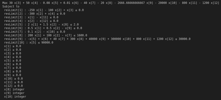
Print a human-readable version of the model in order to check it
ONE POSSIBLE SOLUTION
print(profitModel)12) Optimize the model
ONE POSSIBLE SOLUTION
optimize!(profitModel)13) Check the model resolution status
Check with the function status = termination_status(profitModel) that the status is OPTIMAL (it should be!)
ONE POSSIBLE SOLUTION
status = termination_status(profitModel)14) Print the optimal levels of activities
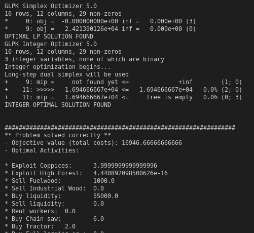
Run the following code to print the results (optimal level of activities):
if (status == MOI.OPTIMAL || status == MOI.LOCALLY_SOLVED || status == MOI.TIME_LIMIT) && has_values(profitModel)
    println("#################################################################")
    if (status == MOI.OPTIMAL)
        println("** Problem solved correctly **")
    else
        println("** Problem returned a (possibly suboptimal) solution **")
    end
    println("- Objective value (total costs): ", objective_value(profitModel))
    println("- Optimal Activities:\n")
    optValues = value.(x)
    for a in 1:nA
      println("* $(activities.label[a]):\t $(optValues[a])")
    end
    if JuMP.has_duals(profitModel)
        println("\n\n- Shadow prices of the resources:\n")
        for r in 1:nR
            println("* $(resources.label[r]):\t $(dual(resLimit[r]))")
        end
    end
else
    println("The model was not solved correctly.")
    println(status)
end
15) [OPTIONAL] Observe the emergence of scale effects
Optionally update the model constraints by using initial2 initial resources (instead of initial) and notice how this larger company can afford to perform different types of activities (logging high forest instead of coppices in this example) and obtain a better profitability per unit of resource employed.
Can you guess which are the aspects of the optimisation model that allow for the emergence of these scale effects?
ONE POSSIBLE SOLUTION
set_normalized_rhs.(resLimit, resources.initial2)
normalized_rhs.(resLimit) # to check the new constraints
optimize!(profitModel)
status = termination_status(profitModel)
if (status == MOI.OPTIMAL || status == MOI.LOCALLY_SOLVED || status == MOI.TIME_LIMIT) && has_values(profitModel)
    println("#################################################################")
    if (status == MOI.OPTIMAL)
        println("** Problem solved correctly **")
    else
        println("** Problem returned a (possibly suboptimal) solution **")
    end
    println("- Objective value (total costs): ", objective_value(profitModel))
    println("- Optimal Activities:\n")
    optValues = value.(x)
    for a in 1:nA
      println("* $(activities.label[a]):\t $(optValues[a])")
    end
    if JuMP.has_duals(profitModel)
        println("\n\n- Shadow prices of the resources:\n")
        for r in 1:nR
            println("* $(resources.label[r]):\t $(dual(resLimit[r]))")
        end
    end
else
    println("The model was not solved correctly.")
    println(status)
end