04 NN - 1A: Introduction and motivations (5:32)
04 NN - 1B: Feed-forward neural networks (18:57)
04 NN - 1C: How to train a neural network (18:4)
04 NN - 1D: Convolutional neural networks (13:21)
04 NN - 1E: Multiple layers in convolutional neural networks (10:33)
04 NN - 1F: Recurrent neural networks (17:49)
0401 - Neural Networks architectures
While powerful, neural networks are actually composed of very simple units that are akin to linear classification or regression methods. Don't be afraid by their name and the metaphor with the human brain. Neural networks are really simple transformations of the data that flow from the input, through various layers, ending with an output. That's their beauty ! Complex capabilities emerge from very simple units when we put them together. For example the capability to recognise not "just" objects in an image but also abstract concepts such as people's emotions or situations and environments.
We'll first describe them, and we'll later learn how to train a neural network from the data. Concerning the practical implementation in Julia, we'll not implement a complete neural network but rather only certain parts, as we will mostly deal with using them and apply them to different kinds of datasets.
Motivations and types
When we studied the Perceptron algorithm, we noted how we can transform the original feature vector $\mathbf{x}$ to a feature representation $\phi(\mathbf{x})$ that includes non-linear transformations, to still use linear classifiers for non-linearly separable datasets (we studied classification tasks but the same is true for regression ones). The "problem" is that this feature transformation is not learned from the data but it is applied a priori, before using the actual machine learning (linear) algorithm. With neural networks instead, the feature transformation is endogenous to the learning (training) step.
We will see three kinds of neural networks:
- Feed-forward Neural Networks, the simplest one where the inputs flow through a set of "layers" to reach an output.
- Convolutional Neural Networks (CNN), where one or more of the layers is a "convolutional" layer. These are used mainly for image classification
- Recurrent Neural Networks (RNN), where the input arrives not only at the beginning but also at each layer. RNNs are used to learn sequences of data
Feed-forward neural networks
Description
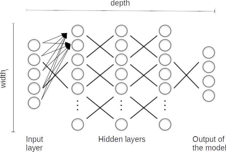
In deep forward neural networks, neural network units are arranged in layers, from the input layer, where each unit holds the input coordinate, through various hidden layer transformations, until the actual output of the model:
More in detail, considering a single dense neuron (in the sense that is connected with all the previous layer's neurons or with the input layer), we have the following figure:
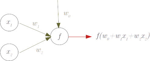
where:
- x is a two-dimensional input, with $x_1$ and $x_2$ being the two dimensions of our input data (they could equivalently be the outputs of a previous 2 neurons layers)
- w are the weigths that are applied to $x$ plus a constant term ($w_0$). These are the parameter we will want to learn with our algorithm. $f$ is a function (often non-linear) that is applied to $w_0 + x_1w_1 + x_2w_2$ to define the output of the neuron
The output of the neuron can be the output of our neural network or it can be the input of a further layer.
In Julia we can implement a layer of neurons and its predictions very easily (although implementing the learning of the weights is a bit more complex):
julia> using LinearAlgebrajulia> mutable struct DenseLayer wb::Array{Float64,1} # weights with reference to the bias (will be learned from data) wi::Array{Float64,2} # weigths with reference to the input (will be learned from data) f::Function # the activation function of each neuron (chosen from the modeller) endjulia> function forward(m,x) # The predictions - or "forward" to the next layer return m.f.(m.wb .+ m.wi * x) endforward (generic function with 1 method)julia> (nI,nO) = 3,2 # Number of nodes in input and in outputs of this layer(3, 2)julia> layer = DenseLayer(rand(nO),rand(nO,nI),tanh)Main.var"Main".DenseLayer([0.9886658021667125, 0.25175894240863705], [0.22882635231244608 0.5353902253325116 0.8469695432047211; 0.3374269685250667 0.6871349196845488 0.8373112676893617], tanh)julia> x = zeros(nI)3-element Vector{Float64}: 0.0 0.0 0.0julia> y = forward(layer,x)2-element Vector{Float64}: 0.7567928440732454 0.24657138069414725
Let's specific a bit of terminology concerning Neural Networks:
- The individual computation units of a layer are known as nodes or neurons.
- Width_l (of the layer) is the number of units in that specific layer $l$
- Depth (of the architecture) is the number of layers of the overall transformation before arriving to the final output
- The weights are denoted with $w$ and are what we want the algorithm to learn.
- Each node's aggregated input is given by $z = \sum_{i=1}^d x_i w_i + w_0$ (or, in vector form, $z = \mathbf{x} \cdot \mathbf{w} + w_0$, with $z \in \mathbb{R}, \mathbf{x} \in \mathbb{R}^d, \mathbf{w} \in \mathbb{R}^d$) and $d$ is the width of the previous layer (or the input layer)
- The output of the neuron is the result of a non-linear transformation of the aggregated input called activation function $f = f(z)$
- A neural network unit is a primitive neural network that consists of only the “input layer", and an output layer with only one output.
- hidden layers are the layers that are not dealing directly with the input nor the output layers
- Deep neural networks are neural network with at least one hidden layer
While the weights will be learned, the width of each layer, the number of layers and the activation functions are all elements that can be tuned as hyperparameters of the model, although there are some more or less formal "rules":
- the input layer is equal to the dimensions of the input data;
- the output layer is equal to the dimensions of the output data. This is typically a scalar in a regression task, but it is equal to the number of categories in a multi-class classification, where each "output dimension" will be the probability associated with that given class;
- the number of hidden layers reflects our judgment on how many "levels" we should decompose our input to arrive at the concept expressed in the label $y$ (we'll see this point dealing with image classification and convolutional networks). Often 1-2 hidden layers are enough for classical regression/classification;
- the number of neurons should give some "flexibility" to the architecture without exploding too much the number of parameters. A rule of thumb is to use about 20% more neurons than the input dimension. This is often fine-tuned using cross-validation as it risks leading to overfitting;
- the activation function of the layers, with the exclusion of the last one, is chosen between a bunch of activation functions, nowadays almost always the Rectified Linear Unit function, aka
relu, defined asrelu(x) = max(0,x). Therelufunction has the advantage to add non-linearity to the transformation while remaining fast to compute (including the derivative) and limiting the problem of vanishing or exploding the gradient (we'll see this aspect when dealing with the actual algorithm to obtain the weights). Another common choice istanh(), the hyperbolic tangent function, that maps with an "S" shape the real line to the interval [-1,1]. - the activation function of the last layer depends on the nature of the labels we want the network to compute: if these are positive scalars we can use also here the
relu, if we are doing a binary classification we can use thesigmoidfunction defined assigmoid(x) = 1/(1+exp(-x))whose output is in the range [0,1] and which we can interpret as the probability of the class that we encode as1. If we are doing a multi-class classification we can use thesoftmaxfunction whose output is a PMF of probabilities for each class. It is defined as $softmax(x,k) = \frac{e^{x_k}}{\sum_{j=1}^{K} e^{x_j}}$ where $x$ is the input vector, $K$ its length and k the specific position of the class for which we want to retrieve its "probability".
Let's now make an example of a single layer, single neuron with a 2D input x=[2,4], weights w=[2,1], w₀ = 2 and activation function f(x)=sin(x).
In such a case, the output of our network is sin(2+2*2+4*1), i.e. -0.54. Note that with many neurons and many layers this becomes essentially (computationally) a problem of matrix multiplications, but matrix multiplication is easily parallelisable by the underlying BLAS/LAPACK libraries or, even better, by using GPU or TPU hardware, and running neural networks (and computing their gradients) is the main reason behind the explosion in the demand of GPU computation.
Let's now assume that the true label that we know to be associated with our $x$ is y=-0.6.
Out (basic) network did pretty well, but still did an error: -0.6 is not -0.54. The last element of a neural network is indeed to define an error metric (the loss function) between the output computed by the neural network and the true label. Commonly used loss functions are the squared l-2 norm (i.e. $\epsilon = \mid \mid \hat y - y \mid\mid ^2$) for regression tasks and cross-entropy (i.e. $\epsilon = - \sum_d p_d * log(\hat p_d)$) for classification jobs.
Before moving to the next section, where we will study how to put everything together and learn how to train the neural network in order to reduce this error, let's first observe that neural networks are powerful tools that can work on many sorts of data, but they require however the input to be encoded in a numerical form, as the computation is strictly numerical. If I have a categorical variable, for example, I'll need to encode it expanding it to a set of dimensions where each dimension represents a single class and I encode with an indicator function if my record is that particular class or not. This is the simplest form of encoding and takes the name of one hot encoding:
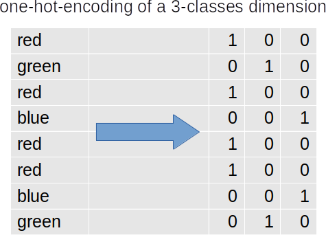
Note in the figure that using all the three columns leads to linearly dependency, and while we could save some resources by using only two columns instead of three, this is not a fundamental problem like it would be in statistical analysis.
Training of a feed-forward neural network
Gradient and learning rate
We now need a way to learn the parameters from the data, and a common way is to try to reduce the contribution of the individual parameter to the error made by the network. We need first to find the link between the individual parameter and the output of the loss function, that is how the error change when we change the parameter. But this is nothing else than the derivative of the loss function with respect to the parameter. In our simple one-neuron example above we have the parameters directly appearing in the loss function. Considering the squared error as lost we have $\epsilon = (y - sin(w_0 + w_1 x_1 + w_2 x_2))^2$. If we are interested in the $w_1$ parameter we can compute the derivate of the error with respect to it using the chain rule as $\frac{\partial\epsilon}{\partial w_1} = 2*(y - sin(w_0 + w_1 x_1 + w_2 x_2)) * - cos(w_0 + w_1 x_1 + w_2 x_2) * x_1$.
Numerically, we have: $\frac{\partial\epsilon}{\partial w_1} = 2(-0.6-sin(2+4+4)) * -cos(2+4+4) * 2 = -0.188$ If I increase $w_1$ of 0.01, I should have my error moving of $-0.01*0.188 = -0.0018$. Indeed, if I compute the original error I have $\epsilon^{t=0} = 0.00313$, but after having moved $w_1$ to 2.01, the output of the neural network chain would now be $\hat y^{t=1} = 0.561$ and its error lowered to $\epsilon^{t=1} = 0.00154$. The difference is $0.00159$, slightly lower in absolute terms than what we computed with the derivate, $0.0018$. The reason, of course, is that the derivative is a concept at the margin, when the step tends to zero.
We should note a few things:
- the derivate depends on the level of $w_1$. "zero" is almost always a bad starting point (as the derivatives of previous layers will be zero). Various initialization strategies are used, but all involve sampling randomly the initial parameters under a certain range
- the derivate depends also on the data on which we are currently operating, $x$ and $y$. If we consider different data we will obtain different derivates
- while extending our simple example to even a few more layers would seem to make the above exercise extremely complex, it remains just an application of the chain rule, and we can compute the derivatives efficiently by making firstly a forward passage, computing (and storing) the values of the chain at each layer, and then making a backward passage by computing (and storing) the derivatives with the chain rule backwards from the last to the first layer
- the fact that the computation of the derivates for a layer includes the multiplication of the derivates for all the other layers means that if these are very small (big) the overall derivate may vanish (explode). This is a serious problem with neural networks and one of the main reasons why simple activation functions such as the
reluare preferred.
The derivate(s) of the error with respect to the various parameters is called the gradient.
If the gradient with respect to a parameter is negative, like in our example, it means that if we slightly increase the parameter we will obtain a lower error. On the opposite, if it is positive, if we slightly reduce the parameter we should find a lower error.
A gradient-descent based algorithm can hence be used to look iteratively for the minimum error by moving against the gradient with a certain step. The most basic algorithm is then $w_i^t = w_i^{t-1} - \frac{\partial\epsilon^{t-1}}{\partial w_1^{t-1}} * \lambda$ where $\lambda$ is the step that you are willing to make against the gradient, also known as learning rate. Note in the example above that if instead of moving the parameter $w_1$ of $0.01$ we would have increased it of $0.1$, we would have increased the error to $0.00997$ instead of reducing it. This highlights the problem to use a good learning rate (see next Figure): a too-small learning rate would make the learning slow and with the risk to get trapped in a local minimum instead of a global one. Conversely, a too-large learning rate would risk causing the algorithm to diverge.
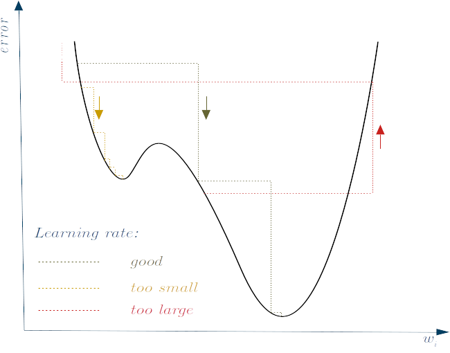
So, the learning rate is also a hyper-parameter to calibrate, although some modern gradient descent variations, like the ADAptive Moment estimation (ADAM) optimisation algorithm, tend to self_tune themselves and we rarely need to calibrate the default values.
Batches and Stochastic gradient descent
We already note that the computation of the gradient depends on the data levels. We can then move between two extremes: on one extreme we compute the gradient as the average of those computed on all data points and we apply the optimisation algorithm to this average. On the other extreme, we sample randomly record by record and, at each record, we move the parameter. The compromise is to partition the data in a set of batches, compute the average gradient of each batch and at each time update the parameter with the optimisation algorithm. The "one record at the time" is the slowest approach, but also is very sensitive to the presence of outliers. The "take the average of all the data" approach is faster in running a certain epoch, but it takes longer to converge (i.e. it requires more epochs, the number of times we pass through the whole training data). It also requires more memory, as we need to store the gradients with respect to all records. So, the "batch" approach is a good compromise, and we normally set the batch number to a multiplier of the number of threads in the machine performing the training, as this step is often parallelised, and it represents a further parameter that we can cross-validate. When we sample the records (individually or in batch) before running the optimisation algorithm we speak of stochastic gradient descent.
Convolutional neural networks
Motivations
Despite typically classified separately, convolutional neural networks are essentially feed-forward neural networks with the only specification that one or more layers are convolutional. These layers are very good at recognising patterns within data with many dimensions, like spatial data or images, where each pixel can be thought a dimension of a single record. In both cases, we could use "normal" feed-forward neural networks, but convolutional layers offer two big advantages:
- They require much fewer parameters.
Convolutional neurons are made of small filters (or kernels) (typically 3x3 or 5x5) where the same weight convolves across the image. Conversely, if we would like to process with a dense layer a mid-size resolution image of $1000 \times 1000$ pixels, each layer would need a weight matrix connecting all these 10^6 pixels in input with 10^6 pixel in output, i.e. 10^12 weights
- They can extend globally what they learn "locally"
If we train a feed-forward network to recognise cars, and it happens that our training photos have the cars all in the bottom half, then the network would not recognise a car in the top half, as these would activate different neurons. Instead, convolutional layers can learn independently on where the individual features apply.
Description
In these networks, the layer $l$ is obtained by operating over the image at layer $l-1$ a small filter (or kernel) that is slid across the image with a step of 1 (typically) or more pixels at the time. The step is called stride, while the whole process of sliding the filter throughout the whole image can be mathematically seen as a convolution.
So, while we slide the filter, at each location of the filter, the output is composed of the dot product between the values of the filter and the corresponding location in the image (both vectorised), where the values of the filters are the weights that we want to learn, and they remain constant across the sliding. If our filter is a $10 \times 10$ matrix, we have only 100 weights to learn by layer (plus one for the offset). Exactly as for feedforward neural networks, then the dot product is passed through an activation function, here typically the ReLU function ($max(0,x)$) rather than tanh:
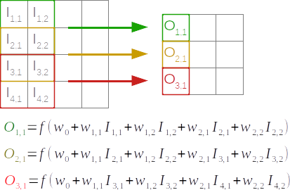
Example
For example, given an image $x = \begin{bmatrix} 1 & 1 & 2 & 1 & 1 \\ 3 & 1 & 4 & 1 & 1 \\ 1 & 3 & 1 & 2 & 2 \\ 1 & 2 & 1 & 1 & 1 \\ 1 & 1 & 2 & 1 & 1 \\ \end{bmatrix}$ and filter weights $w = \begin{bmatrix} 1 & -2 & 0 \\ 1 & 0 & 1 \\ -1 & 1 & 0 \\ \end{bmatrix}$, then the output of the filter $z$ would be $\begin{bmatrix} 8 & -3 & 6 \\ 4 & -3 & 5 \\ -3 & 5 & -2 \\ \end{bmatrix}$. For example, the element of this matrix $z_{2,3} = 5$ is the result of the sum of the scalar multiplication between $x^\prime = \begin{bmatrix} 4 & 1 & 1 \\ 1 & 2 & 2 \\ 1 & 1 & 1 \\ \end{bmatrix}$ and $w$.
Finally, the output of the layer would be (using ReLU) $\begin{bmatrix} 8 & 0 & 6 \\ 4 & 0 & 5 \\ 0 & 5 & 0 \\ \end{bmatrix}$.
We can run the following snippet to make the above computations:
julia> ReLU(x) = max(0,x)ReLU (generic function with 1 method)julia> x = [1 1 2 1 1; 3 1 4 1 1; 1 3 1 2 2; 1 2 1 1 1; 1 1 2 1 1]5×5 Matrix{Int64}: 1 1 2 1 1 3 1 4 1 1 1 3 1 2 2 1 2 1 1 1 1 1 2 1 1julia> w = [ 1 -2 0; 1 0 1; -1 1 0]3×3 Matrix{Int64}: 1 -2 0 1 0 1 -1 1 0julia> (xr,xc) = size(x)(5, 5)julia> (wr,wc) = size(w)(3, 3)julia> z = [sum(x[r:r+wr-1,c:c+wc-1] .* w) for c in 1:xc-wc+1 for r in 1:xr-wr+1] # Julia is column major9-element Vector{Int64}: 8 4 -3 -3 -3 5 6 5 -2julia> u = ReLU.(z)9-element Vector{Int64}: 8 4 0 0 0 5 6 5 0julia> final = reshape(u, xr-wr+1, xc-wc+1)3×3 Matrix{Int64}: 8 0 6 4 0 5 0 5 0
You can notice that by applying the filter we obtain a dimensionality reduction. This reduction depends on both the dimension of the filter and the stride (sliding step). In order to avoid this, padding of one or more rows/columns can be applied to the image to preserve in the output the same dimension of the input (in the above example padding of one row and one column on both sides would suffice). Typically, the padded cells are given a value of zero so not to contribute anything when they are included in the dot product computed by the filter.
To determine the spatial size in the output of a filter ($O$), given the input size ($I$), the filter size ($F$), the stride ($S$) and the eventual padding ($P$) we can use the following simple formula:
\[O_d = 1 + (I_d+2*P_d-F_d)/S\]
From it, we can also find the padding needed to obtain a certain output size as: $P_d = ((O_d-1)S_d-I_d+F_d)/2$
Where the $d$ index accounts for the (extremely unusual) case where one of the parameters is not a square matrix so that for example an image has different vertical and horizontal resolutions.
Because the weights of the filters are the same, it doesn't really matter where the object is learned, in which part of the image. With convolutional layers, we have translational invariance as the same filter is passed over the entire image. Therefore, it will detect the patterns regardless of their location.
Still, it is often convenient to operate some data augmentation to the training set, that is to add slightly modified images (rotated, mirrored...) in order to improve this translational invariance.
Considering multiple filters per layer
Typically, one single layer is formed by applying multiple filters, not just one. This is because we want to learn different kinds of features. For example in an image one filter will specialize to catch vertical lines, the other obliques ones, and maybe another filter different colours.
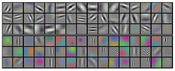
Convolutional filters outputs on the first layer (filters are of size 11x11x3 and are applied across input images of size 224x224x3). Source: Krizhevsky et Oth. (2012), "ImageNet Classification with Deep Convolutional Neural Networks"
So in each layer we map the output of the previous layer (or the original image in case of the first layer) into multiple feature maps where each feature map is generated by a little weight matrix, the filter, that defines the little classifier that's run through the original image to get the associated feature map. Each of these feature maps defines a channel for information and we can represent it as a third dimension to form a "volume", where the depth is given by the different filters:
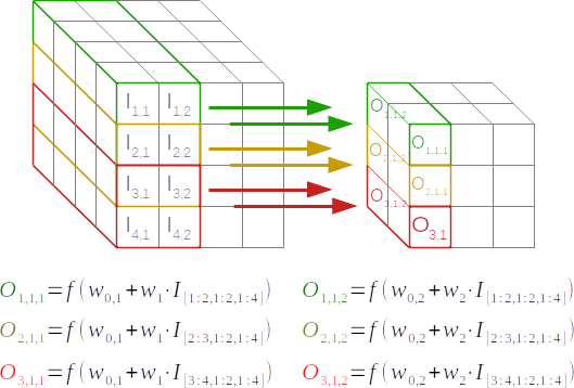
In the image above the input layer has size (4,4,4) and the output layer has size (3,3,2), i.e. 2 "independent" filters of size (2,2).
For square layers, each filter has $F^2 \times D_{l-1} + 1$ parameters where $D_{l-1}$ is the dimensions ("depth") of the previous layer, so the total number of parameters per layer is $(F^2 \times D_{l-1} + 1) * D_l$.
For computational reasons, the number of filters per layer $D_l$ is normally a power of 2.
This representation allows remaining consistent with the input that can as well be represented as a volume. For images, the depth is usually given by 3 layers representing the values in terms of RGB colours.
Pool layers
A further way to improve translational invariance, but also have some dimensionality reduction, is called pooling and is implemented by adding a layer with a filter whose output is the max of the corresponding area in the input (or, more rarely, the average). Note that this layer would have no weights to learn! With pooling we start separating what is in the image from where it is in the image, that is, pooling does a fine-scale, local translational invariance, while convolution does more a large-scale one.
Keeping the output of the above example as input, a pooling layer with a $2 \times 2$ filter and a stride of 1 would result in $\begin{bmatrix} 8 & 6 \\ 5 & 5 \\ \end{bmatrix}$.
Convolutional networks conclusions
We can then combine these convolutions, looking for features, and pooling, compressing the image a little bit, forgetting the information of where things are, but maintaining what is there.
In a typical CNN, these convolutional and pooling layers are repeated several times, where the initial few layers typically would capture the simpler and smaller features, whereas the later layers would use information from these low-level features to identify more complex and sophisticated features, like characterisations of a scene. The learned weights would hence specialise across the layers in a sequence like edges -> simple parts-> parts -> objects -> scenes.
These layers are finally followed by some "normal", "fully connected" layers (like in "normal" feed-forward neural networks) and a final softmax layer indicating the probability that each image represents one of the possible categories (there could be thousands of them).
The best network implementations are tested in so-called "competitions", like the yearly ImageNet context.
Note that we can train these networks exactly like for feedforward NN, defining a loss function and finding the weights that minimise the loss function. In particular, we can apply the stochastic gradient descendent algorithm (with a few tricks based on getting pairs of image and the corresponding label), where the gradient with respect to the various parameters (weights) is obtained by backpropagation.
Recurrent Neural Networks (RNNs)
Motivations
Recurrent neural networks are used to learn sequences of data. A "sequence" is characterised by the fact that each element may depend not only on the features in place at time $t$, but also from lagged features or lagged values of the sequence (we use here the time dimension just for simplicity. Of course, a sequence can be defined on any dimension). And here comes the problem: we could always consider lagged features or sequence values as further dimensions at time $t$ and use a "standard" feed-forward network. For example, we could consider values at time $t-1$, those at time $t-2$ and those at time $t-3$. But, again, we would be doing "manual" feature engineering, similar to the way we can introduce non-linear feature transformation and use linear classifiers. But we want this to be learned by the algorithm. We want the model to learn how much of the history retain to predict the next element of the sequence, and which elements "deserve" to be kept in memory (to be used for predictions) even if far away in the sequence steps.
Description
There are a few differences with feed-forward neural networks:
- the input doesn't arrive only at the beginning of the chain, but at each layer (each input being an element of the sequence)
- each RNN layer processes, using learnable parameters, the input corresponding to its layer, together the input coming from the previous layers (called the state)
- these weights are shared for the various RNN layers across the sequence
Note that you can interpret a recurrent network equivalently like being formed by different layers on each element of the sequence (but with shared weights) or like a single, evolving, layer that calls itself recursively. Note also the similarities with convolutional networks: there we have a filter than convolves along the image, keeping the weigths constant across the convolution, here we have a recurrent network that also "filter" the whole sequence and learn some shared weigths.
To implement a recurrent neural network we can adapt our code above to include the state:
julia> mutable struct RNNLayer wb::Array{Float64,1} # weights with reference to the bias wi::Array{Float64,2} # weigths with reference to the input ws::Array{Float64,2} # weigths with reference to the state f::Function endjulia> (nI,nO) = 3,2(3, 2)julia> relu(x) = max(0,x)relu (generic function with 1 method)julia> rnnLayer = RNNLayer(rand(nO),rand(nO,nI),rand(nO,nO),relu)Main.var"Main".RNNLayer([0.009793771133059681, 0.2451738630886735], [0.7587955942199099 0.8883291034342745 0.3984675606303608; 0.8366312917809341 0.6807782629269769 0.20984799792849484], [0.09607171363771372 0.6863957018710027; 0.5394538922089241 0.21081248135790054], Main.var"Main".relu)julia> function forward(m,x,s) return m.f.(m.wb .+ m.wi * x .+ m.ws * s) endforward (generic function with 2 methods)julia> x,s = zeros(nI),zeros(nO)([0.0, 0.0, 0.0], [0.0, 0.0])julia> s = forward(rnnLayer,x,s)2-element Vector{Float64}: 0.009793771133059681 0.2451738630886735julia> s = forward(rnnLayer,x,s) # The state change even if x remains constant2-element Vector{Float64}: 0.17902096134396348 0.30214286148763136
The code above is the simplest implementation of a Recurrent Neural Network (or at least of its forward passage). In practice, the state is often memorised as part of the layer structure so its usage in most neural network libraries is similar to a "normal" feed-forward layer forward(layer,x).
Usage: sequence-to-one
RNNs can be used to characterise a sequence, like in sentiment analysis to predict the overall attitude (positive or negative) of a text or the language in which the text is written. In these cases, the RNN task is to encode the sequence in a vector format (the final state) and this is fed to a further part of the chain whose task is to decode according to the task required. Note that the parameters for both tasks are learned jointly. The scheme is as follow:
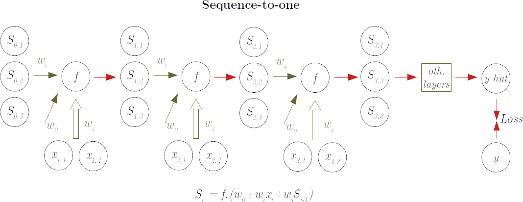
Training in this scenario implies starting the model from an initial state (normally a zero-vector) and some random weights, and "feeding" the model with one item at a time until the sequence ends. At this time the final state is decoded to an overall output that is compared to the "true" y. From here the backward passage is made in a similar way that in feed-forward networks so that the "contribution" of each weight to the errors can be assessed and the weights adjusted
While weights are progressively adjusted across the training samples, the state of the network should be reset at each new sequence sample.
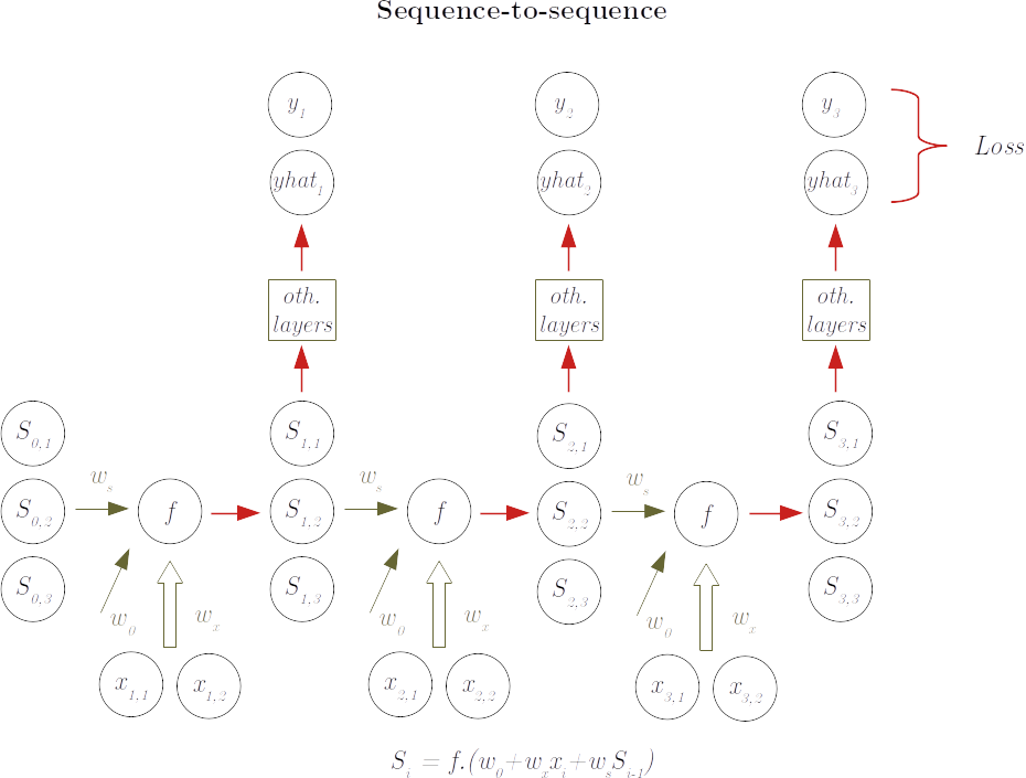
Usage: sequence-to-sequence
Another scenario is when we want the RNN to replicate some sequence pattern, like in next word, next note or next price predictions. In this case, we are interested in all the elements of the sequence and not only in the final state of the sequence. The decoding part happens hence at each step of the sequence and the resulting $\hat y_i$ is compared with the true $y_i$, with the resulting loss used to train the weights:
Gated networks
While theoretically RNN can "learn" the importance of features across indeterminately long sequence steps, in practice the fact of continuing multiplicating the status across the varius elements of the sequence makes the problem of vanishing gradient even stronger for them. New contributions have hence been proposed with a "gating" system that "learns" what to store in memory (in the sequence state) and what to "forget". At the time of writing the most used approach is the Long short-term memory (LSTM). While internally more complex due to the presence of the gates and of several different states (hidden and visible in LSTM), LSTM networks are operationally used exactly in the same ways as the RNN networks described above.